2025-07-17

Step-by-Step Diffusion: An Elementary Tutorial

Nakkiran, Preetum, Arwen Bradley, Hattie Zhou, and Madhu Advani. “Step-by-Step Diffusion: An Elementary Tutorial.” arXiv, June 23, 2024. https://doi.org/10.48550/arXiv.2406.08929.

Fundamental of Diffusion
Stochastic Sampling: DDPM
Deterministic Sampling: DDIM
Flow Matching
Diffusion in Practice
Further Reading and Resources

1. Fundamental of Diffusion

Goal of Generative Modelling: Given i.i.d. samples from an unknown distribution \(p^*\), we create a method that can generate new samples by sampling from an approximation of \(p^*(x)\).

i.i.d. samples: Independent and identically distributed samples

Each sample was drawn independently and all samples come from same underlying distribution \(p^*\).

Example: We have a training set of 10,000 dog photos:

These photos represent samples from some true distribution \(p_{dog}(x)\) over all possible dog images and we don’t know the mathematical form of \(p_{dog}(x)\)
Our goal is to create a system that can generate new, realistic dog images that look like they could have come from the same distribution

Idea: Learn a transformation from some easy-to-sample distribution (such as Gaussian noise) to our target distribution \(p^*\).

Diffusion models offer a general framework for learning such transformations.
The clever trick of diffusion is to reduce the problem of sampling from distribution \(p^{*}(x)\) into to a sequence of easier sampling problems.

1.1 Gaussian Diffusion

Forward Pass

Systematically transforms target data (like images of dogs) into pure noise through a series of small, random steps.

Starting point: We have some data \(x_0\) sampled from target distribution \(p^*\) (e.g., real dog images).

The forward process: You create a sequence \(x_0 \rightarrow x_1 \rightarrow x_2 \rightarrow \ldots \rightarrow x_T\) by repeatedly adding small amounts of Gaussian noise:

\[x_{t+1} = x_t + \eta_t, \quad \text{where } \eta_t \sim \mathcal{N}(0, \sigma^2)\]

This means each step adds independent Gaussian noise with variance \(\sigma^2\).

Final state: After \(T\) steps, the distribution \(p_T\) becomes approximately Gaussian \(\mathcal{N}(0, \sigma^2)\).

This happens because we are repeatedly adding independent Gaussian noise and the Central Limit Theorem ensures that the result approaches a Gaussian distribution. Variance grows linearly with the number of steps.

\[\text{(See figure below)}\]

Images as 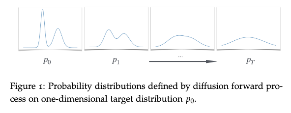420

So we can approximately sample from \(p_T\) by just sampling a Gaussian.
We can directly sample \(x_t\) given \(x_0\) without computing all intermediate steps. (Sum of Gaussians is Gaussian)

Reverse Sampling

Strategy

The authors propose to solve generative modelling by decomposing it into many simpler “reverse sampling” steps:

Instead of: Learning to generate samples from \(p^*\) directly (very hard)
Do this: Learn to go backwards one step at a time: \(p_T \rightarrow p_{T-1} \rightarrow p_{T-2} \rightarrow \ldots \rightarrow p_0 = p^*\)

Why This Decomposition Helps

The key insight is that adjacent distributions (\(p_{t-1}, p_t\)) are very similar because we only add a small amount of noise \(\sigma\) at each step. This makes the reverse step much easier to learn than the full generative problem.

Think of it like this:

Hard: Transform pure noise into a realistic dog image in one step
Easy: Remove a tiny bit of noise from an almost-clean dog image

The DDPM Reverse Sampler

DDPM: Denoising Diffusion Probabilistic Models

The “obvious” approach is to learn the conditional distribution \(p(x_{t-1} \mid x_t)\) for each step. Given a noisy sample \(x_t\), we want to predict what the slightly less noisy version \(x_{t-1}\) should be.

Fact 1: When \(\sigma\) is small, the conditional distribution \(p(x_{t-1} \mid x_t)\) is approximately Gaussian.

This means:

\[p(x_{t-1} \mid x_t = z) \approx \mathcal{N}(\mu_{t-1}(z), \sigma^2)\]

So instead of learning an arbitrary complex distribution, we only need to learn the mean function \(\mu_{t-1}(z)\).

\[\text{(See figure below)}\]

Images as 421

The Regression Formulation

Since we know the distribution is Gaussian with known variance \(\sigma^2\), learning the mean is equivalent to solving a regression problem:

\[\mu_{t-1} = \arg\min \mathbb{E}\left[\|f(x_t) - x_{t-1}\|^2\right]\]

This can be rewritten as:

\[\mu_{t-1} = \arg\min \mathbb{E}\left[\|f(x_{t-1} + \eta_t) - x_{t-1}\|^2\right]\]

where \(\eta_t \sim \mathcal{N}(0, \sigma^2)\) is the noise we added.

Theorem: For any joint distribution over random variables \((X, Y)\), the conditional expectation \(\mathbb{E}[Y \mid X]\) is the function that minimizes the mean squared error:

\[\mathbb{E}[Y \mid X] = \arg\min_{f} \mathbb{E}\left[(f(X) - Y)^2\right]\]

The Beautiful Connection to Denoising

Notice what this regression objective is asking: given a clean signal \(x_{t-1}\) plus some noise \(\eta_t\), predict the original clean signal.

This is exactly the image denoising problem! We can use standard denoising techniques (like convolutional neural networks) to solve it.

The authors have reduced the complex problem of generative modeling to the well-understood problem of regression/denoising.

Instead of learning to generate realistic images from scratch, we learn to remove small amounts of noise—doing this many times in sequence to gradually transform pure noise into realistic samples.

This is why diffusion models work so well: they break down an impossibly hard problem into many manageable denoising steps that neural networks are already good at solving.

1.2 Diffusions in the Abstract

Diffusion models follow a universal pattern that works across many different settings—not just Gaussian noise, but also discrete domains, deterministic processes, and more.

Discrete Domains: Instead of working with continuous values (like pixel intensities 0.0 to 1.0), we work with discrete, finite sets of possibilities. For example, text generation where each position can be one of a finite vocabulary.
Deterministic Processes: The reverse sampler produces the same output every time you give it the same input—there’s no randomness involved.

The Abstract Recipe

Step 1: Choose your endpoints

Start with target distribution \(p^*\) (what you want to generate)
Choose a base distribution \(q\) that’s easy to sample from (e.g., Gaussian noise, random bits)

Step 2: Create an interpolating sequence

Build a sequence of distributions that smoothly connects these endpoints:

\[p_0 = p^* \rightarrow p_1 \rightarrow p_2 \rightarrow \ldots \rightarrow p_T = q\]

The key requirement is that adjacent distributions (\(p_{t-1}, p_t\)) are “close” in some meaningful sense.

Step 3: Learn reverse samplers

For each step \(t\), learn a function \(F_t\) that can transform samples from \(p_t\) back to \(p_{t-1}\).

The Reverse Sampler Definition

This is the formal definition of what we need to learn:

Definition: A reverse sampler \(F_t\) is a function such that if you:

Take a sample \(x_t\) from distribution \(p_t\)
Apply \(F_t\) to get \(F_t(x_t)\)
The result is distributed according to \(p_{t-1}\)

Mathematically:

\[F_t(z) : z \sim p_t \implies F_t(z) \sim p_{t-1}\]

Why This Abstraction is Powerful

Flexibility: This framework works for:

Continuous domains (images with Gaussian noise)
Discrete domains (text, categorical data)
Deterministic processes (no randomness in the reverse step)
Stochastic processes (with randomness)

Multiple implementations: The same abstract framework gives us:

DDPM (stochastic, Gaussian-based)
DDIM (deterministic version)
Flow-matching (continuous-time generalization)

The Key Insight About “Closeness”

The magic happens because adjacent distributions are “close.” This means:

The reverse sampling step \(F_t\) doesn’t need to do much work
Learning becomes feasible because we’re making small adjustments rather than dramatic transformations

The Coupling Perspective

Given the marginal distributions \({p_t}\), there are many possible ways to define the joint relationships between consecutive steps. These are called “couplings” in probability theory.

This means we have freedom in how we design the reverse sampler—we can choose whichever coupling is most convenient for learning or sampling.

Why This Matters

This abstraction shows that diffusion models aren’t just about “adding noise”—they’re about:

Interpolation: Creating smooth paths between complex and simple distributions
Decomposition: Breaking hard problems into many easier steps
Flexibility: Adapting the same core idea to many different domains and applications

1.3 Discretisation

We need to be more precise about what we mean by adjacent distributions \(p_t\), \(p_{t-1}\) being “close”.

The Continuous-Time Perspective

The authors are shifting from thinking about discrete steps (\(x_0\), \(x_1\), \(x_2\), …) to a continuous-time process \(p(x,t)\) where:

\(t = 0\): We have our target distribution \(p^*\)
\(t = 1\): We have our base distribution (noise)
\(t \in [0,1]\): We have intermediate distributions

The discrete steps are just a discretisation of this continuous process:

\[p_k(x) = p(x, k \cdot \Delta t) \qquad \text{where} \; \Delta t = 1/T\]

Finer discretisation = closer adjacent distributions:

Large \(T \rightarrow\) small \(\Delta t \rightarrow\) many small steps \(\rightarrow\) adjacent distributions are very close
Small \(T \rightarrow\) large \(\Delta t \rightarrow\) few big steps \(\rightarrow\) adjacent distributions are farther apart

This explains why diffusion models work better with more steps!

The Variance Scaling Problem and \(\sqrt{\Delta t}\) Scaling

Here’s a subtle but crucial issue: If we naively add noise \(\sigma^2\) at each step, then after \(T\) steps we’d have total variance \(T \cdot \sigma^2\). This means:

More steps \(\rightarrow\) higher final variance
Fewer steps \(\rightarrow\) lower final variance

But we want the final distribution to be the same regardless of how many steps we take.

Solution

To fix this, they scale the noise variance by \(\Delta t\):

\[\sigma = \sigma_q \sqrt{\Delta t} = \sigma_q \sqrt{1/T}\]

Why this works: After \(T\) steps, the total variance becomes:

\[\text{Total variance} = T \times \sigma_q^2 \Delta t = T \times \sigma_q^2 \times (1/T) = \sigma_q^2\]

So regardless of \(T\), the final variance is always \(\sigma_q^2\)!

The New Notation

This scaling ensures that as \(T \rightarrow \infty\) (continuous limit), the process converges to a well-defined continuous-time stochastic process.

From now on:

t represents continuous time in \([0,1]\), not discrete steps
\(\Delta t = 1/T\) is the step size
\(x_t\) means “x at time t” (not “x at step t”)

The forward process becomes:

\[x_{t+\Delta t} = x_t + \eta_t, \qquad \text{where} \; \eta_t \sim N(0, \sigma_q^2 \Delta t)\]

The Cumulative Effect

\[x_t \sim N(x_0, \sigma_t^2) \qquad \text{where} \; \sigma_t := \sigma_q \sqrt{t}\]

This beautiful formula shows that:

At \(t = 0\): \(\sigma_0 = 0\) (no noise, original data)
At \(t = 1\): \(\sigma_1 = \sigma_q\) (full noise level)
At \(t = 0.5\): \(\sigma_{0.5} = \sigma_q \sqrt{0.5}\) (intermediate noise)

This discretization framework:

Unifies discrete and continuous views of diffusion
Ensures consistency across different numbers of steps
Enables theoretical analysis of the continuous limit
Connects to stochastic differential equations (SDEs)

2. Stochastic Sampling: DDPM

This section introduces the DDPM (Denoising Diffusion Probabilistic Models) sampler - the classic stochastic approach to diffusion sampling. Let me break this down:

The DDPM sampler learns to predict what the previous (less noisy) timestep looked like given the current (more noisy) timestep. Specifically, it learns:

\[\mu_t(z) := E[x_t \mid x_{t+\Delta t} = z]\]

This means: “Given that we observe value \(z\) at time \(t+\Delta t\), what was the expected value at the previous time \(t\)?”

The Training Process

Objective: Learn the conditional expectation functions \({\mu_t}\) by solving a regression problem:

\[\mu_t = \arg\min \; E[||f(x_{t+\Delta t}) - x_t||^2]\]

What this means:

Take pairs of (\(x_t\), \(x_{t+\Delta t}\)) from the forward diffusion process
Train a neural network to predict the cleaner version \(x_t\) given the noisier version \(x_{t+\Delta t}\)
This is literally a denoising problem!

Practical implementation: Instead of learning separate functions for each timestep, we typically train a single neural network \(f_\theta(x, t)\) that takes both the noisy sample and the time \(t\) as input.

Sampling Algorithm 1: Stochastic Reverse Sampler (DDPM-like Sampler)

Once trained, the reverse sampler works as follows:

For input sample \(x_t\), and timestep \(t\), output:

\[\hat{x}_{t-\Delta t} \leftarrow \mu_{t-\Delta t}(x_t) + N(0, \sigma_q^2 \Delta t)\]

Breaking this down:

\(\mu_{t-\Delta t}(x_t)\): Use the learned function to predict the mean of the previous timestep
\(+ N(0, \sigma_q^2 \Delta t)\): Add Gaussian noise with the same variance as the forward process
The result is a sample from the previous timestep

The Full Generation Process

Step 1: Start with pure noise: \(x_1 \sim N(0, \sigma_q^2)\)
Step 2: Apply Algorithm 1 repeatedly:

\[x_1 \rightarrow x_{1-\Delta t} \rightarrow x_{1-2\Delta t} \rightarrow ... \rightarrow x_0\]

Step 3: The final \(x_0\) is your generated sample

Why This Works (Conceptually)

The magic relies on Fact 1: that the true conditional distribution \(p(x_{t-\Delta t} \mid x_t)\) is approximately Gaussian when \(\Delta t\) is small.
If this is true, then:
- We only need to learn the mean \(\mu_{t-\Delta t}(x_t)\) (since we know the variance is \(\sigma_q^2 \Delta t\))
- We can sample from this conditional by taking the predicted mean plus Gaussian noise
- Each step undoes a small amount of the forward corruption

The Stochastic Nature

Notice that this sampler is stochastic - even if you start with the same noise \(x_1\), you’ll get different samples \(x_0\) because of the added noise at each step. This is different from deterministic samplers like DDIM.

2.1 Correctness of DDPM: Look in paper for the proof

The Problem: We needed to prove that DDPM’s reverse sampler actually works - that it can successfully generate samples from our target distribution.

The Key Question: Why is the reverse process (going from noisy to clean) approximately Gaussian?

The Answer:

Used Bayes’ rule to express the reverse conditional probability \(p(x_{t-\Delta t} \mid x_t)\)
Applied Taylor expansion around the current point
Completed the square to show it has Gaussian form

The Result:

\[p(x_{t-\Delta t} \mid x_t) = N(\text{mean}, \sigma_q^2 \Delta t)\]

where the mean involves the “score” (gradient of log probability).

Why This Matters:

Since the reverse process is Gaussian, we only need to learn its mean
Learning the mean is just a regression problem (predicting clean from noisy)
This justifies why DDPM works: each reverse step is a simple denoising operation

The Bottom Line: DDPM works because when you add small amounts of noise, reversing that process is approximately Gaussian, which makes it learnable through standard regression techniques.

2.2 Algorithms

Pseudocode 1: DDPM Training

What it does: Trains the neural network to do denoising regression.

Step by step:

Get clean data: Sample \(x_0\) from target distribution (e.g., real images)
Pick random time: Sample \(t\) uniformly from \([0,1]\)
Add noise up to time t: Create \(x_t = x_0 + N(0, \sigma_q^2 t)\)
Add one more step of noise: Create \(x_{t+\Delta t} = x_t + N(0, \sigma_q^2 \Delta t)\)
Train to denoise: \(\text{Loss} = \left\| f_\theta(x_{t+\Delta t}, t+\Delta t) - x_t \right\|^2\)

Key insight: The network learns to predict the cleaner version \(x_t\) given the noisier version \(x_{t+\Delta t}\) and the time \(t+\Delta t\).

Pseudocode 2: DDPM Sampling

What it does: Generates new samples using the trained model.

Step by step:

Start with pure noise: \(x_1 \sim N(0, \sigma_q^2)\)
Go backwards in time: For \(t = 1, 1-\Delta t, 1-2\Delta t, ..., \Delta t\)
Predict + add noise: \(x_{t-\Delta t} = f_\theta(x_t, t) + N(0, \sigma_q^2 \Delta t)\)
Return final result: \(x_0\) is your generated sample

Key insight: Each step predicts the cleaner version, then adds noise to account for uncertainty (this is the stochastic part).

Pseudocode 3: DDIM Sampling (Preview)

What it does: Deterministic version of sampling (no added noise).

Key difference: Instead of adding random noise, it uses a deterministic update rule with a mixing coefficient \(\lambda\).

Important Notes

Training is simultaneous: The network learns to denoise at ALL timesteps at once.
Sampling goes backwards: We go from \(t=1\) (pure noise) to \(t=0\) (clean data)
Same network for all steps: \(f_\theta(x,t)\) handles all timesteps using the time input \(t\)

2.3 Variance Reduction: Predicting \(x_0\)

This section explains an important practical trick used in diffusion models! Let me break it down:

The Two Training Approaches

Original approach: Train the network to predict \(E[x_{t-\Delta t} \mid x_t]\) - the previous timestep
Alternative approach: Train the network to predict \(E[x_0 \mid x_t]\) - the original clean data

Why This Works (Claim 2):

We have:

\[E[(x_{t-\Delta t} - x_t) \mid x_t] = \frac{\Delta t}{t} E[(x_0 - x_t) \mid x_t]\]

and its equivalent to:

\[E[x_{t-\Delta t} \mid x_t] = \left(\frac{\Delta t}{t}\right) E[x_0 \mid x_t] + \left(1 - \frac{\Delta t}{t}\right) x_t\]

This means: if you can predict the clean image \(x_0\), you can easily compute what the previous timestep \(x_{t-\Delta t}\) should be.

The Intuitive Explanation

The noise symmetry argument:

When you observe \(x_t\), it’s the sum: \(x_0 + \eta_1 + \eta_2 + \ldots + \eta_t\) (all the noise steps)
You can’t tell which noise came from which step—they all “look the same”
So instead of predicting one noise step \(\eta_{t-\Delta t}\), you can predict the average of all noise steps
The average has much lower variance than individual steps!

Why This is Better (Variance Reduction)

Problem with predicting \(x_{t-\Delta t}\): You’re trying to estimate one noisy step from another noisy observation—high variance.

Solution with predicting \(x_0\): You’re averaging over all the noise steps, which reduces variance significantly.

Think of it like this:

High variance: “Given this noisy image, what did the slightly less noisy version look like?”
Low variance: “Given this noisy image, what did the original clean image look like?”

The second question is easier because you’re not trying to distinguish between very similar noise levels.

Important Warning

Critical point: The model predicts \(E[x_0 \mid x_t]\), which is the expected value, not a sample!

What this means:

If you’re generating faces, \(E[x_0 \mid x_t]\) might be a blurry average of all possible faces
It won’t look like a real face—it’s a mathematical expectation
This is normal and expected!

Common misconception: People think “predicting \(x_0\)” means the model outputs something that looks like a real sample. It doesn’t—it outputs the average of all possible samples.

Practical Implementation

In practice:

Train the model to predict \(E[x_0 \mid x_t]\) (better variance)
During sampling, use the relationship in Claim 2 to convert this back to \(E[x_{t-\Delta t} \mid x_t]\)
Apply the sampling algorithm as usual

The Mathematical Relationship

The division by \(\left(\frac{t}{\Delta t}\right)\) in the formula represents the number of steps taken so far. Since we’ve accumulated \(\left(\frac{t}{\Delta t}\right)\) noise steps, we divide the total predicted noise by this amount to get the average per step.

3. Deterministic Sampling: DDIM

DDIM: Denoising Diffusion Implicit Model → A deterministic alternative to the stochastic DDPM sampler.

Algorithm 2: Deterministic Reverse Sampler (DDIM-like)

Instead of using the stochastic sampler that adds random noise at each step, DDIM uses a deterministic function that always produces the same output for the same input.

For input sample \(x_t\), and step index \(t\), output:

\[\hat{x}_{t-\Delta t} = x_t + \lambda \left( \mu_{t-\Delta t}(x_t) - x_t \right)\]

Where:

\[\lambda = \frac{\sigma_t}{\sigma_{t-\Delta t} + \sigma_t}\]

and

\[\sigma_t = \sigma_q \sqrt{t}\]

\(\mu_{t-\Delta t}(x_t) = E[x_{t-\Delta t} \mid x_t]\) is the conditional expectation (what we’d predict on average)
\(\lambda = \frac{\sigma_t}{\sigma_{t-\Delta t} + \sigma_t}\) is a scaling factor
\(\sigma_t = \sigma_q \sqrt{t}\) from the noise schedule

Understanding the Formula

Let’s interpret what this update is doing:

Step 1: \(\mu_{t-\Delta t}(x_t) - x_t\)

This is the “direction” we need to move to get from the current noisy sample to the predicted less-noisy sample.

Step 2: \(\lambda (\mu_{t-\Delta t}(x_t) - x_t)\)

We scale this direction by factor \(\lambda\). This determines how far we actually move.

Step 3: \(x_t + \lambda (\mu_{t-\Delta t}(x_t) - x_t)\)

We take a step in that direction from our current position.

Why This Scaling Factor \(\lambda\)?

The scaling factor \(\lambda\) has a nice interpretation:

When \(\sigma_{t-\Delta t} \approx \sigma_t\) (small time step), then \(\lambda \approx \frac{1}{2}\) (take a moderate step)
When \(\sigma_{t-\Delta t} \ll \sigma_t\) (large time step), then \(\lambda \approx 1\) (take the full predicted step)
When \(\sigma_{t-\Delta t} \gg \sigma_t\) (this shouldn’t happen in forward process), then \(\lambda \approx 0\)

Deterministic vs Stochastic

DDPM (Stochastic):

Samples from \(p(x_{t-\Delta t} \mid x_t)\)
Same input can give different outputs
Adds randomness at each step

DDIM (Deterministic):

Uses a fixed function \(F_t(x_t)\)
Same input always gives same output
No randomness in the reverse process

The Transport Map Perspective

Instead of thinking about sampling from conditional distributions, DDIM thinks about transport maps—functions that transform one distribution into another.

The goal is to show that the function \(F_t\) defined by the DDIM update “pushes” the distribution \(p_t\) to \(p_{t-\Delta t}\):

\[F_t \,\sharp\, p_t \approx p_{t-\Delta t}\]

The notation \(F\,\sharp\,p\) means “the distribution you get when you apply function \(F\) to samples from distribution \(p\)”.

Advantages of DDIM:

Faster sampling: Can take bigger steps since it’s deterministic
Reproducible: Same starting noise always gives same result
Interpolation: Can smoothly interpolate between samples
Fewer steps: Often works well with far fewer steps than DDPM

Connection to other methods: This deterministic approach connects to flow-matching and other continuous-time methods.

We need to Prove that DDIM is correct and works:

The authors will prove this works by:

Point-mass case: Show it works for the simplest distributions (single points)
Marginalization: Extend to full distributions by considering all possible points

This is similar to how flow-matching methods are analyzed—by showing the transport map works pointwise and then extending to distributions.

The key insight is that even though we’re not sampling from \(p(x_{t-\Delta t} \mid x_t)\), we can still achieve the same marginal distribution \(p_{t-\Delta t}\) through this deterministic transport.

3.1 Case 1: Single Point

Avoiding complicated math: Refer to paper

What are we trying to prove?

We want to show that DDIM (the deterministic sampler) actually works. But proving it for complicated distributions is hard, so we start with the simplest possible case.

The simplest case: One dot

Imagine our target is just a single dot at position 0. That’s it—we want to generate samples that are exactly at position 0.

What happens when we add noise?

Start: We have a dot at position 0
After some time: The dot has moved randomly and is now somewhere else (due to noise)
Our job: Figure out how to move it back toward 0

The obvious solution

If we know the dot started at 0, and now it’s at some noisy position, the obvious thing to do is shrink it back toward 0.
If the dot is currently at position 10, and we know it should be closer to 0, we should move it to maybe position 7 or 5 (somewhere closer to 0).

The key insight

The fancy DDIM formula is actually just doing this simple shrinking!

\[\text{New position} = \text{Old position} + \lambda (\text{Predicted position} - \text{Old position})\]

But in the simple case, this reduces to:

\[\text{New position} = (\text{shrink\_factor}) \times \text{Old position}\]

Where \(\text{shrink_factor}\) is less than 1, so we’re moving the dot closer to 0.

Why this matters

This proves that DDIM works correctly in the simplest case. It’s doing exactly what we’d expect—gradually shrinking the noise to bring samples back to the target.

The bigger picture

DDIM looks complicated with all its formulas and Greek letters
But in the simplest case, it’s just gradually shrinking noisy samples back toward the target
This gives us confidence that it’s doing something sensible in more complex cases too

Think of it like this: if you wanted to guide a lost person back to their house, you’d tell them to walk in the direction of their house. DDIM is doing the same thing—it’s figuring out which direction to move to get closer to the target, then taking a step in that direction.

3.2 Velocity Fields and Gases

Instead of thinking about DDIM as a mathematical formula, we can think of it as a velocity field—like wind patterns that tell particles which way to move.

The DDIM update can be rewritten as:

\[\hat{x}_{t-\Delta t} = x_t + v_t(x_t) \cdot \Delta t\]

Where:

\[v_t(x_t) = \frac{\lambda}{\Delta t} \left( E[x_{t-\Delta t} \mid x_t] - x_t \right)\]

This looks just like physics: position = old position + velocity × time!

The Gas Analogy

Imagine a gas made of particles:

Each particle represents a possible sample
The density of particles at any location represents the probability of that sample
The gas starts with density pattern \(p_t\) (more spread out/noisy)
We want it to end up with density pattern \(p_{t-\Delta t}\) (less spread out/noisy)

How the Velocity Field Works

The velocity field \(v_t(x)\) tells each particle at position \(x\) which direction to move:

Direction: Toward where that particle “should” be (based on \(E[x_{t-\Delta t} \mid x_t]\))
Speed: Proportional to how far it needs to move

When all particles move according to this velocity field, the overall gas density transforms from \(p_t\) to \(p_{t-\Delta t}\).

Note: Skipping Proofs

3.3 Case 2: Two Points

3.4 Case 3: Arbitrary Distributions

3.5 The Probability Flow ODE [Optional]

3.6 Discussion: DDPM vs DDIM

DDPM (Stochastic):

Takes a sample and produces a random output from \(p(x_{t-\Delta t} \mid x_t)\)
Same input can give different outputs each time

DDIM (Deterministic):

Takes a sample and produces the same output every time
Creates a fixed mapping from input to output

The Iteration Behaviour

When you run these algorithms from start to finish, they behave very differently:

DDPM: Independence from Starting Point

Key insight: If you start DDPM from different initial noise samples \(x_1\), you’ll get samples that are essentially independent of where you started.
Why: The forward process “mixes” well—it scrambles the original data so much that the final noise \(x_1\) contains almost no information about the original \(x_0\).
Result: \(p(x_0 \mid x_1) \approx p(x_0)\)—the output doesn’t depend on the starting noise!
Analogy: Like shuffling a deck of cards so thoroughly that the final order tells you nothing about the original order.

DDIM: Strong Dependence on Starting Point

Key insight: DDIM creates a deterministic function from noise to data.
Why: Since it’s deterministic, the same starting noise \(x_1\) always produces the same final output \(x_0\).
Result: Different starting points lead to different, but predictable outputs.
Analogy: Like having a specific recipe—same ingredients always give the same dish.

The Mapping Perspective

This reveals something profound about DDIM:

DDIM as a Special Map

What it does: Creates a deterministic function from Gaussian noise \(\rightarrow\) target distribution
Sounds familiar: This is similar to GANs and Normalizing Flows, which also map noise to data. But there’s a key difference… The Constraint Makes It Special
- GANs: Can learn any mapping that works—complete freedom
- DDIM: Must learn the specific mapping determined by the target distribution
Why this matters:
- Supervised vs Unsupervised: DDIM has a “correct answer” to learn toward
- Smoothness: The DDIM map inherits smoothness from the target distribution
- Structure: The mapping respects the geometry of the data

Practical Implications

DDPM Advantages:

Sample diversity: Randomness can help explore different modes
Robustness: Less sensitive to the exact starting point

DDIM Advantages:

Reproducibility: Same noise always gives same result
Interpolation: Can smoothly interpolate between samples
Speed: Often works with fewer steps
Control: Deterministic nature enables better control

The Learning Trade-off

Easier aspects of DDIM:

Has a “ground truth” target function to learn
Inherits nice properties from the target distribution
Supervised learning setup

Harder aspects of DDIM:

Must learn the specific “correct” mapping
Less flexibility than arbitrary mappings
May miss easier-to-learn alternatives

Visual Intuition

DDPM: Like a skilled artist who can paint many different dogs from the same reference photo—each painting is different but all are valid dogs.
DDIM: Like a precise photocopier that always produces the exact same copy from the same input—deterministic but perfectly reproducible.

The Philosophical Difference

DDPM: “Generate samples that look like they came from the target distribution”
DDIM: “Learn the specific transformation that the diffusion process implies”

This fundamental difference in philosophy leads to all the practical differences we observe in how these methods behave!

3.7 Remarks on Generalization

This section addresses a crucial practical issue that often gets overlooked in theoretical discussions of diffusion models: How do we actually learn these models from real data without just memorizing the training set?

The Core Problem

What we want: A model that learns the underlying distribution and can generate new, similar samples.

What we might get: A model that just memorizes the training data and can only reproduce exact copies of what it saw.

The Empirical Risk Minimization Trap

Standard approach: Train by minimizing prediction error on the training set.

The problem: If we minimize this error perfectly, we get a model that:

Perfectly predicts the training data
Only generates samples that are exactly from the training set
Never creates anything genuinely new

Why this fails: Perfect memorization of finite training data doesn’t help us learn the true underlying distribution.

Imagine learning to draw dogs:

Bad approach: Memorize every pixel of 1000 dog photos and only reproduce those exact photos
Good approach: Learn what makes something “dog-like” and generate new dog images

The Regularization Solution

The key insight: We need to prevent perfect memorization through regularization.

Explicit regularization: Add penalties to prevent overfitting
Implicit regularization: Natural limitations prevent memorization:

Finite model capacity: The neural network can’t memorize everything
Optimization randomness: SGD doesn’t find the perfect memorizing solution
Early stopping: We don’t train to perfect convergence

Why This Matters

For researchers: Understanding that perfect optimization isn’t the goal—we want controlled generalization.
For practitioners:
- Larger datasets help prevent memorization
- Some “imperfection” in training is actually beneficial
- Need to balance fitting the data vs. generalizing

The Security/Copyright Issue

Real concern: Models trained on copyrighted or private data might reproduce it exactly.
Evidence: Researchers have shown they can extract training images from models like Stable Diffusion with carefully crafted prompts.

Practical Takeaways

Don’t aim for perfect training loss—some generalization error is good
Use larger datasets when possible to reduce memorization
Implicit regularization from neural network training often helps naturally
Be aware of privacy/copyright implications of potential memorization

4 Flow Matching

Flow matching is a generalization of DDIM that provides much more flexibility in designing generative models.

The core ideas behind DDIM don’t actually require:

Gaussian noise
The specific Gaussian forward process
Any particular base distribution

Instead, the fundamental concept is about transporting distributions using vector fields.

The Two-Step Construction from DDIM

Looking back at how DDIM worked, there were really two key steps:

Step 1: Point-to-Point Transport

For any single target point \(a\), we can construct a vector field \(v[a]_t\) that transports a sample from the base distribution (like standard Gaussian) to exactly that point \(a\).

Think of this as: “How do I move a particle from random noise to land exactly at point \(a\)?”

Example:

Target point \(a\) = “golden retriever sitting”
Vector field \(v[a]_t\) = instructions for how to move a noise sample to become exactly this image

Step 2: Combining Vector Fields

When we have multiple target points (or a whole distribution), we combine the individual vector fields into a single effective vector field.

This is like: “If I want to transport noise to match a complex distribution, I combine the ‘instructions’ for reaching each individual point.”

Example: If we have many target points, we need to combine all these individual vector fields into one unified vector field that can generate the entire distribution.

\(v[a_1]_t\) → path to “golden retriever sitting”
\(v[a_2]_t\) → path to “beagle running”
\(v[a_3]_t\) → path to “poodle sleeping”
etc.

\[v_t(x) = \int v[a]_t(x) \cdot p^*(a) \, da\]

Or in discrete terms:

\[v_t(x) = \sum v[a]_t(x) \cdot P(\text{target} = a)\]

What This Means Intuitively

At any point \(x\) and time \(t\), the combined vector field tells you:

“Move in the direction that’s the average of all individual directions”
“Weight each direction by how likely that target is in your dataset”

Suppose at some point \(x\) during the denoising process:

\(v[a_1]_t(x)\) says “move right” (toward golden retriever)
\(v[a_2]_t(x)\) says “move left” (toward beagle)
\(v[a_3]_t(x)\) says “move up” (toward poodle)

And your dataset has:

50% golden retrievers
30% beagles
20% poodles

Then the combined vector field would be:

\[v_t(x) = 0.5 \times \text{"right"} + 0.3 \times \text{"left"} + 0.2 \times \text{"up"}\]

The Learning Process

In practice, we don’t know all the individual vector fields \(v[a]_t\) ahead of time. Instead:

Sample pairs: Take samples \((x_0, x_1)\) where \(x_0\) is from base distribution and \(x_1\) is from target distribution
Construct path: For each pair, define a path from \(x_0\) to \(x_1\) (like a straight line)
Learn average: Train a neural network to predict the average velocity along all these paths

Connection to DDIM

In DDIM, this combination happens implicitly:

The conditional expectation \(E[x_{t-\Delta t} \mid x_t]\) is already the result of combining all possible paths
The Gaussian assumptions make this combination mathematically tractable
The vector field emerges from the denoising objective

The Generalization

Flow matching asks: What if we drop all the Gaussian assumptions?

Instead of being limited to:

Gaussian base distributions
Gaussian forward processes
Specific noise schedules

We can now think about:

Any two points \(x_0\) and \(x_1\)
Any two distributions \(p\) (data) and \(q\) (base)
Any smooth path connecting them

Why This Matters

In traditional diffusion models (DDPM/DDIM), the paths are curved because of how Gaussian noise is added and removed.

Why curved? The forward process adds noise gradually: clean \(\rightarrow\) slightly noisy \(\rightarrow\) more noisy \(\rightarrow\) pure noise. The reverse process follows the same curved trajectory backwards.

Imagine a ball rolling down a curved hill—it doesn’t go straight down, it follows the curved surface.

More flexible paths: Instead of the specific curved paths that Gaussian diffusion creates, we can design:

1. Straight lines (rectified flows)

Instead of curved paths, we connect each noise sample to its corresponding data sample with a straight line.

If you start at noise point \(x_1\) and want to reach data point \(x_0\):

\[x(t) = (1-t)x_1 + t \cdot x_0\]

Why this is better:

Faster sampling: Straight lines are the shortest distance between two points
Fewer steps needed: You can take bigger steps along a straight path
More predictable: Easier to control and understand
Less computation: Simpler math than curved trajectories

Used in Stable Diffusion 3: This makes SD3 faster and more efficient than previous versions.

2. Custom trajectories

Design paths that are optimized for your specific data type or use case.

Like For images:

Paths that preserve image structure early in generation
Trajectories that handle different frequency components separately
Paths optimized for specific image types (faces, landscapes, etc.)

For text:

Paths that maintain syntactic structure while changing semantics
Trajectories that respect language hierarchies (words \(\rightarrow\) sentences \(\rightarrow\) paragraphs)

For 3D shapes:

Paths that preserve geometric constraints
Trajectories that respect physical laws (like gravity for fluid simulations)

For audio:

Paths that preserve harmonic structure
Trajectories optimized for different types of sounds (speech, music, etc.)

3. Paths that avoid low-probability regions

This is a sophisticated optimization that’s really powerful:

The problem: In high-dimensional spaces, there are regions where data almost never appears. Traditional diffusion might accidentally pass through these “impossible” regions.

Example with faces:

Low-probability region: Images with eyes in impossible positions, or faces that morph unnaturally
Good path: Stays in regions that look like plausible faces throughout the generation process

Visual analogy: Imagine you’re hiking from point A to point B. You could:

Take a straight line (might go through dangerous cliffs)
Take a curved path that stays on safe, well-traveled trails

How it works:

Instead of: noise \(\rightarrow\) weird intermediate states \(\rightarrow\) final image
Design: noise \(\rightarrow\) always plausible-looking states \(\rightarrow\) final image

Benefits:

Better intermediate results: Every step looks reasonable
More stable training: Less likely to get stuck in impossible configurations
Higher quality: Final results are more realistic
Conditional generation: Better control over the generation process

Different base distributions:

We’re not limited to Gaussian noise. We could use:

Uniform distributions
Other structured noise patterns
Even data-dependent base distributions

Broader applications:

This framework works for:

Continuous data (images, audio)
Discrete data (with appropriate metrics)
Structured data (graphs, molecules)
Any domain where you can define smooth interpolation

The Mathematical Framework

The core mathematical object is a vector field \(v_t(x)\) that tells you:

At time \(t\)
At position \(x\)
Which direction and how fast to move

The flow is generated by solving the ODE:

\[\frac{dx}{dt} = v_t(x)\]

Modern Applications

Conditional flows: Generate samples conditioned on additional information (text, class labels, etc.)

This framework has become the foundation for many state-of-the-art generative models because of its flexibility and mathematical elegance.

4.1 Flows

This section formalizes the mathematical foundation of flows.

What is a Flow?

A flow is a collection of time-indexed vector fields:

\[v = \{ v_t \}_{t \in [0,1]}\]

Think of it as a velocity field that tells particles how to move at each point in space and time.

Physical analogy: Imagine a river with currents. At each location \((x, y)\) and time \(t\), the current has a specific velocity and direction. The flow tells you: “If you’re at position \(x\) at time \(t\), move in direction \(v_t(x)\).”

The Flow ODE

Any flow defines how particles move via the differential equation:

\[\frac{dx}{dt} = -v_t(x_t)\]

Starting condition: Begin at \(x_1\) at time \(t = 1\)
Ending condition: End at \(x_0\) at time \(t = 0\)

Note the negative sign: This is because time runs backwards from 1 to 0 (following diffusion convention where \(t=0\) is clean data).

RunFlow Function

The \(\text{RunFlow}(v, x_1, t)\) function solves the ODE and tells you:

Input: Starting point \(x_1\), flow \(v\), target time \(t\)
Output: Where the particle ends up at time \(t\)

Intuitive meaning: “If I start at \(x_1\) and follow the flow \(v\), where will I be at time \(t\)?”

Flows don’t just move individual points—they transport entire distributions:

Individual point: \(x_1 \rightarrow \text{RunFlow}(v, x_1, 0) = x_0\)
Entire distribution: \(p_1 \rightarrow p_0\)

The Ultimate Goal

We want to learn a flow \(v^*\) such that:

\[q \xrightarrow{v^*} p\]

Where:

q: Easy-to-sample base distribution (like Gaussian noise)
p: Target distribution (like dog images)
v: The optimal flow that connects them

Generation Process

Once we have \(v^*\), generating samples is simple:

Sample: \(x_1 \sim q\) (sample from base distribution)
Transport: \(x_0 = \text{RunFlow}(v^*, x_1, 0)\) (follow the flow)
Output: \(x_0\) (this is your generated sample)

Connection to DDIM

DDIM is actually a special case of flow matching!

DDIM’s flow: The continuous-time limit of DDIM corresponds to the flow:

\[v_t(x_t) = \frac{1}{2t} E[x_0 - x_t \mid x_t]\]

Components:

Base distribution: Gaussian
DDIM sampling: Discretized method for evaluating RunFlow
DDPM training: Method for learning \(v^*\) (but relies on Gaussian structure)

4.2 Pointwise Flows

Core idea: A pointwise flow connects one specific point \(x_1\) to one specific point \(x_0\).

What it does: Given any path from \(x_1\) to \(x_0\), the pointwise flow describes the velocity at each point along that path.

Mathematical definition: \(v^{[x_1, x_0]}\) is a flow that satisfies the ODE with boundary conditions:

Starts at \(x_1\) when \(t = 1\)
Ends at \(x_0\) when \(t = 0\)

Key insight: Pointwise flows are not unique. You can choose different paths between the same two points: straight line, curved path, any smooth trajectory.

4.3 Marginal Flows

The problem: We have many individual pointwise flows, but we need one unified flow that handles the entire distribution.

The setup:

Pick a coupling \(\Pi_{q,p}\) (way to pair noise samples with data samples)
For each pair \((x_1, x_0)\), use pointwise flow \(v^{[x_1, x_0]}\)
This gives us a “collection of particle trajectories”

The solution: Combine all pointwise flows into one marginal flow \(v^*\) using weighted averaging:

\[v^*_t(x_t) = E[ v^{[x_1, x_0]}_t(x_t) \mid x_t ]\]

Intuitive meaning: At any point \(x_t\) and time \(t\), the marginal flow velocity is the average velocity of all particles that happen to be at \(x_t\) at that time.

Why this works:

Individual particles follow their own pointwise flows
The bulk behavior emerges from averaging all individual behaviors
Result: one flow that transports \(q \rightarrow p\)

Gas analogy: Instead of tracking every individual gas particle, we describe the bulk fluid motion—the average velocity at each location.

Remaining challenges:

Which pointwise flow to choose? (straight lines? curves?)
How to compute \(v\) in practice?

These questions drive the practical algorithms we’ll see next.

4.4 A Simple Choice of Pointwise Flow

The Three Design Choices

To build a flow matching model, we need to choose:

Base distribution \(q\): What we sample from initially
1. Gaussian (most common)
2. Uniform
3. Annular (ring-shaped)
Coupling \(\Pi_{q,p}\): How we pair base samples with target samples. Independent sampling—just sample from \(p\) and \(q\) separately and pair them randomly.
Pointwise flow: How we connect each pair

Linear Pointwise Flow

The simplest pointwise flow is straight-line interpolation:

\[v^{[x_1, x_0]}_t(x_t) = x_0 - x_1\]

This gives a constant velocity pointing from \(x_1\) to \(x_0\).

The resulting trajectory:

\[\text{RunFlow}(v^{[x_1, x_0]}, x_1, t) = t x_1 + (1-t) x_0\]

This is just linear interpolation between the two points!

At different times \(t\):

\(t = 1\): Position is \(x_1\) (base distribution sample)
\(t = 0.5\): Position is \(0.5 x_1 + 0.5 x_0\) (halfway between)
\(t = 0\): Position is \(x_0\) (target distribution sample)

Physical interpretation: A particle moves at constant speed from \(x_1\) to \(x_0\), taking exactly 1 time unit to complete the journey.

4.5 Flow Matching

We want to compute the optimal vector field \(v^*_t(x_t)\), but naively this requires sampling from \(p(x_0 \mid x_t)\)—which is exactly the hard problem we’re trying to solve! It’s circular reasoning.

The DDPM Trick Applied to Flow Matching

Just like in DDPM, we can avoid this circular problem by using regression:

Instead of trying to sample from \(p(x_0 \mid x_t)\), we:

Sample from the joint distribution \((x_0, x_1)\)—this is easy!
Compute \(x_t\) deterministically using our chosen flow
Set up a regression problem to learn the expected vector field

The key insight is that:

\[v^*_t(x_t) = E[ v^{[x_1, x_0]}_t(x_t) \mid x_t ]\]

And by the fundamental regression theorem:

\[v^*_t = \arg\min_f E\left[ \| f(x_t) - v^{[x_1, x_0]}_t(x_t) \|^2 \right]\]

This means we can learn \(v^*_t\) by minimizing squared error!

The Training Process

Pseudocode 4: Flow-matching train loss, generic pointwise flow [or linear flow]

\[\text{(See figure below)}\]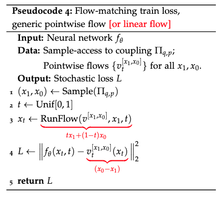

420

Let me walk through each step:

Step 1: \((x_1, x_0) \leftarrow \text{Sample}(\Pi_{q,p})\)

Sample a source point \(x_1\) from base distribution \(q\) (e.g., Gaussian noise)
Sample a target point \(x_0\) from data distribution \(p\) (e.g., real image)
These form a training pair

Step 2: \(t \leftarrow \text{Unif}[0, 1]\)

Pick a random time point during the flow

Step 3: \(x_t \leftarrow \text{RunFlow}(v^{[x_1, x_0]}, x_1, t)\)

Starting from \(x_1\), run the pointwise flow for time \(t\) to get \(x_t\)
For linear flows: \(x_t = t \cdot x_1 + (1-t) \cdot x_0\)

Step 4: \(L \leftarrow \| f_\theta(x_t, t) - v^{[x_1, x_0]}_t(x_t) \|^2\)

\(f_\theta(x_t, t)\): What our neural network predicts the velocity should be
\(v^{[x_1, x_0]}_t(x_t)\): What the true velocity should be for this specific flow
For linear flows: \(v^{[x_1, x_0]}_t(x_t) = x_0 - x_1\)

The Sampling Process

Pseudocode 5: Flow-matching sampling

\[\text{(See figure below)}\]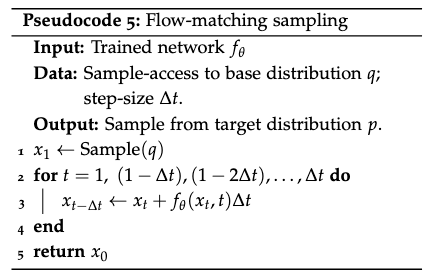

420

Step 1: \(x_1 \leftarrow \text{Sample}(q)\)

Start with a random sample from the base distribution (noise)

Steps 2-4: Iterative integration

For each time step, update: \(x_{t-\Delta t} \leftarrow x_t + f_\theta(x_t, t) \Delta t\)
This is Euler integration of the ODE \(\frac{dx}{dt} = f_\theta(x, t)\)
We’re following the learned vector field from noise to data

The Beautiful Simplicity: This framework is elegant because:

No complex probability calculations—just regression
Flexible path design—choose any pointwise flow you want
Efficient sampling—straightforward ODE integration
Scalable training—standard neural network optimization

The key insight is that by breaking the problem into pointwise flows and then learning their average, we can solve generative modeling using simple, well-understood techniques.

https://mlg.eng.cam.ac.uk/blog/2024/01/20/flow-matching.html: helpful visualizations of flows, and uses notation more consistent with the current literature.

5 Diffusion in Practice

Samplers in Practice

The Speed Problem

DDPM and DDIM samplers are essentially the “Model T” of diffusion sampling. Each sampling step requires an expensive neural network forward pass, and even today’s best samplers need around 10 steps minimum.
This is a massive bottleneck. Imagine waiting 10+ seconds for a single image generation when users expect near-instantaneous results.

The SDE/ODE Connection Unlocks Better Samplers

Since DDPM and DDIM are discretizations of the reverse SDE and Probability Flow ODE respectively, we can leverage decades of numerical methods research.

Any ODE/SDE solver becomes a potential diffusion sampler:

Euler methods
Heun’s method
Runge-Kutta variants
Custom solvers designed for diffusion’s specific structure

This perspective transformed sampler development from ad-hoc tweaking to principled numerical analysis.

The Distillation Revolution

Distillation methods that train student models to match multi-step diffusion teachers in just one step:

Consistency Models
Adversarial Distillation

⚠️ Important caveat: These distilled models aren’t technically diffusion models anymore—they’re neural networks trained to mimic diffusion output, but they’ve abandoned the iterative denoising process entirely.

Noise Schedules

Why Schedules Matter

The noise schedule (\(\sigma_t\)) determines how much noise gets added at each timestep. This seemingly simple choice has profound implications for training stability, sample quality, and convergence speed.

Variance Exploding vs. Variance Preserving

Simple diffusion has \(p(x_t) \sim N(x_0, \sigma_t^2)\) with \(\sigma_t \propto \sqrt{t}\), meaning variance explodes over time. This is one of two major paradigms:

Variance Exploding (VE): Noise variance grows unboundedly
Variance Preserving (VP): Noise variance stays controlled

The Ho et al. Schedule (Still Industry Standard)

The most popular schedule comes from the original DDPM paper:

\[x_t = \sqrt{1 - \beta(t)} \cdot x_{t-1} + \sqrt{\beta(t)} \cdot \varepsilon_t\]

Where \(\beta(t)\) is carefully chosen so that:

\(t = 1\): Nearly clean data
\(t = 1\): Pure noise
Variance remains bounded throughout

The Karras Reparameterization

Karras et al. [2022] introduced a more intuitive way to think about schedules using:

Overall scaling: \(s(t)\)
Variance: \(\sigma(t)\)

Their suggested schedule: \(s(t) = 1, \sigma(t) = t\)

This framework makes it much easier to reason about and experiment with different noise schedules.

The SDE Framework: Maximum Flexibility

The general SDE formulation gives us incredible flexibility:

\[dx_t = f(x_t, t)dt + g(t)dw_t\]

Examples of what this enables:

Our simple diffusion: \(f = 0\), \(g = \sigma_q\)
Ho et al. schedule: \(f = -\frac{1}{2}\beta(t)\), \(g = \sqrt{\beta(t)}\)
Karras schedule: \(f = 0\), \(g = \sqrt{2t}\)

Likelihood Interpretations and VAEs.

Diffusion as Hierarchical VAE

Here’s a perspective that fundamentally changed how we think about diffusion models: they’re actually a special case of deep hierarchical VAEs. This isn’t just theoretical elegance—it has profound practical implications.

The key insight: Each diffusion timestep corresponds to one “layer” of a VAE decoder, with the forward diffusion process acting as a fixed (non-learned) encoder that produces the sequence of noisy latents \(\{x_t\}\).

Why This Perspective Revolutionized Training

Traditional deep VAEs suffer from notorious training instability because gradients must flow through all layers. Diffusion’s Markovian structure breaks this dependency—each layer can be trained in isolation without forward/backward passing through previous layers.

This is why diffusion models train so much more stably than traditional deep generative models.

The Likelihood Advantage

The VAE interpretation gives us something incredibly valuable: actual likelihood estimates via the Evidence Lower Bound (ELBO). This means we can train diffusion models with principled maximum-likelihood objectives.

Plot twist: The ELBO for diffusion VAEs reduces to exactly the L2 regression loss we’ve been using, but with specific time-weighting that treats regression errors differently at different timesteps.

⚠️ The practical dilemma: The “principled” VAE-derived time-weighting doesn’t always produce the best samples. Ho et al. [2020] famously just dropped the time-weighting and uniformly weighted all timesteps—sometimes theory and practice diverge!

Parametrization: The \(x_0\) / \(\varepsilon\) / \(v\)-Prediction Wars

What Should Your Network Actually Predict?

This is one of the most important practical decisions you’ll make, and it’s not obvious. You have three main options:

1. Direct Prediction (What We’ve Been Doing)

\[\min \| f_\theta(x_t, t) - x_{t-\Delta t} \|^2\]

Network predicts the partially-denoised data.

2. \(x_0\)-Prediction

\[\min \| f_\theta(x_t, t) - x_0 \|^2\]

Network predicts the fully-denoised original data. This is nearly equivalent to direct prediction, differing only by a time-weighting factor of \(1/t\).

3. \(\varepsilon\)-Prediction

\[\min \| f_\theta(x_t, t) - \varepsilon_t \|^2\]

Network predicts the noise that was added. Where \(\varepsilon_t = (1/\sigma_t) E[x_0 - x_t \mid x_1]\).

4. \(v\)-Prediction
Network predicts \(v = \alpha_t \varepsilon - \sigma_t x_0\)—essentially predicting data at high noise levels and noise at low noise levels.

Why This Choice Matters Enormously

Mathematically, these are equivalent—they differ only by time-weightings. In practice, they behave very differently because:

Learning is imperfect—certain objectives may be more robust to errors
Different parametrizations have different failure modes
Some combinations are fundamentally problematic

Example failure case: \(x_0\)-prediction with schedules that heavily weight low noise levels often fails because the identity function achieves low loss but produces terrible samples.

The Error Landscape: What Actually Goes Wrong

Training-Time Errors

These are standard statistical learning errors in approximating the population-optimal regression function:

Approximation error: Your network architecture isn’t expressive enough
Estimation error: You don’t have enough training data
Optimization error: Your training procedure doesn’t find the global optimum

Sampling-Time Errors

These are discretization errors from using finite step-sizes \(\Delta t\):

For DDPM: Error in the Gaussian approximation of the reverse process
For DDIM/Flow Matching: Error in simulating continuous-time flows discretely

The Interaction Problem

Here’s what makes this challenging: these errors interact and compound in complex, poorly understood ways. We don’t fully understand how regression errors translate into distributional errors of the final generative model.

Surprising twist: These “errors” can actually be beneficial on small datasets, acting as regularization that prevents the model from just memorizing training samples.

Key Practical Takeaways

VAE Perspective Guides Training Strategy: Understanding diffusion as hierarchical VAE explains why they train so stably and provides principled likelihood-based objectives (even if you sometimes ignore the principled weighting).
Parametrization Choice Is Critical: The \(x_0\)/\(\varepsilon\)/\(v\)-prediction choice significantly impacts training dynamics and sample quality. There’s no universal best choice—it depends on your specific use case and schedule.
Error Sources Are Inevitable But Manageable: Both training-time and sampling-time errors are unavoidable, but understanding their sources helps you make informed trade-offs between speed, quality, and robustness.
Theory vs. Practice Tension: The “principled” choices from theory don’t always win in practice. Be prepared to empirically validate theoretical insights rather than blindly following them.

420

Step-by-Step Diffusion: An Elementary Tutorial

Table of Contents

1. Fundamental of Diffusion

1.1 Gaussian Diffusion

Forward Pass

Reverse Sampling

The DDPM Reverse Sampler

1.2 Diffusions in the Abstract

The Abstract Recipe

The Reverse Sampler Definition

Why This Abstraction is Powerful

The Key Insight About “Closeness”

The Coupling Perspective

1.3 Discretisation

The Continuous-Time Perspective

The Variance Scaling Problem and \(\sqrt{\Delta t}\) Scaling

The New Notation

2. Stochastic Sampling: DDPM

The Training Process

Sampling Algorithm 1: Stochastic Reverse Sampler (DDPM-like Sampler)

More

2.1 Correctness of DDPM: Look in paper for the proof

2.2 Algorithms

Pseudocode 1: DDPM Training

Pseudocode 2: DDPM Sampling

Pseudocode 3: DDIM Sampling (Preview)

Important Notes

2.3 Variance Reduction: Predicting \(x_0\)

The Two Training Approaches

Why This Works (Claim 2):

The Intuitive Explanation

Why This is Better (Variance Reduction)

Important Warning

Practical Implementation

The Mathematical Relationship

3. Deterministic Sampling: DDIM

Algorithm 2: Deterministic Reverse Sampler (DDIM-like)

Understanding the Formula

Why This Scaling Factor \(\lambda\)?

Deterministic vs Stochastic

The Transport Map Perspective

Advantages of DDIM:

We need to Prove that DDIM is correct and works:

3.1 Case 1: Single Point

3.2 Velocity Fields and Gases

The Gas Analogy

How the Velocity Field Works

Note: Skipping Proofs

3.6 Discussion: DDPM vs DDIM

The Iteration Behaviour

The Mapping Perspective

Practical Implications

The Learning Trade-off

Visual Intuition

The Philosophical Difference

3.7 Remarks on Generalization

The Core Problem

The Empirical Risk Minimization Trap

The Regularization Solution

Practical Takeaways

4 Flow Matching

The Two-Step Construction from DDIM

Step 1: Point-to-Point Transport

Step 2: Combining Vector Fields

The Generalization

Why This Matters

1. Straight lines (rectified flows)

2. Custom trajectories

3. Paths that avoid low-probability regions

Different base distributions:

Broader applications:

The Mathematical Framework

Modern Applications

4.1 Flows

The Flow ODE

RunFlow Function

The Ultimate Goal

Generation Process

Connection to DDIM

4.2 Pointwise Flows