Stable Audio - Fast Timing-Conditioned Latent Audio Diffusion
Evans, Zach, C. J. Carr, Josiah Taylor, Scott H. Hawley, and Jordi Pons. “Fast Timing-Conditioned Latent Audio Diffusion.” arXiv:2402.04825. Preprint, arXiv, May 13, 2024. https://doi.org/10.48550/arXiv.2402.04825.
Model-Code - Metrices - Demo
Table of Contents
1 Summary
The Problem with Audio Diffusion
Raw audio is massive in size and complexity. That means:
- Training is slow and memory-intensive.
- Inference (actually generating audio) is even slower, especially for long clips or stereo output.
- Another practical issue: most audio diffusion models only generate fixed-length clips.
- A model trained on 30-second chunks will always give you exactly 30 seconds — even when your prompt suggests something shorter or longer. This is unnatural, especially for:
- Music, which has structure (like intros and outros)
- Sound effects, which can be quick or long
- A model trained on 30-second chunks will always give you exactly 30 seconds — even when your prompt suggests something shorter or longer. This is unnatural, especially for:
Stable Audio
- A convolutional VAE that efficiently compresses and reconstructs long stereo audio.
- It uses latent diffusion — meaning it learns to denoise in a compressed, lower-dimensional space (the latent space), not on raw audio. This is much faster and allows for longer generation.
- It adds timing embeddings — so you can tell the model how long the output should be.
That combo allows it to:
- Generate up to 95 seconds of full-quality audio in just 8 seconds
- Offer precise control over the duration and content
- Render stereo audio at 44.1kHz — the same sample rate used in CDs
Rethinking Audio Evaluation
- Fréchet Distance with OpenL3: Measures how realistic the audio sounds by comparing it to real-world audio using perceptual embeddings.
- KL Divergence: Quantifies how well the semantic content of the generated audio matches a reference.
- CLAP Score: Assesses how well the generated audio aligns with the text prompt.
They also go a step further by assessing:
- Musical structure (does it feel like a song, or just a loop?)
- Stereo correctness (do the left and right channels make sense?)
- Human perception (via qualitative studies)
2 Related Work
2.1 Autoregressive Models: Great Sound, Painfully Slow
What they are:
Autoregressive models generate audio one step (or token) at a time. Think of it like writing a sentence word by word — each decision depends on what came before.
Examples:
- WaveNet (2016): Generated audio from scratch using raw waveform values — high-quality but painfully slow.
- Jukebox (2020): Compressed music into multi-scale latent tokens, then used transformers to model them.
- MusicLM / MusicGen / AudioLM: Modern versions that use text prompts instead of artist/genre metadata and work on compressed audio tokens.
Problem: Even with compression, these models are slow to generate audio because of their step-by-step nature.
2.2 Non-Autoregressive Models: Faster, Still Limited
What they are:
These models try to speed up generation by skipping the step-by-step process.
Examples:
- Parallel WaveNet, GAN-based methods: Tried adversarial training.
- VampNet / MAGNeT / StemGen: Use masked modeling (like BERT) or other tricks to avoid sequential generation.
- Flow-matching models: Try to morph noise into data in a more direct way.
Problem: Many are limited in the duration they can handle (up to 20 seconds) or don’t focus on structured or stereo music.
2.3 Diffusion Models
- End-to-End Diffusion: These generate raw waveforms directly (e.g., CRASH, DAG, Noise2Music). Powerful, but training is costly and slow.
- Spectrogram Diffusion: Generate images of sound (spectrograms) and convert them back to waveforms.
- Riffusion: Generated audio by tweaking Stable Diffusion for spectrograms.
- Needs a separate vocoder (like HiFi-GAN) to reconstruct audio.
- Latent Diffusion (Stable Audio’s Approach)
- Moûsai, AudioLDM, JEN-1: All use VAE-based latents to make the job easier and faster.
- AudioLDM: Generates spectrograms first, then inverts to audio.
- Moûsai: Diffuses latents and directly decodes into audio.
- JEN-1: A multitask model with dimensionality-reduced latents.
- Stable Audio’s Differentiator: Also uses latent diffusion, but focuses on 44.1kHz stereo audio, supports up to 95 seconds, and introduces timing conditioning — something none of these others do.
2.4 High Sampling Rate & Stereo Audio
Most past models:
- Work in mono or low sample rates (16–24kHz).
- Or generate short clips.
Only a few (e.g., Moûsai, JEN-1) can handle stereo and high quality — but not efficiently, and not with variable length.
Stable Audio’s edge: One of the first models to combine:
- 44.1kHz stereo
- Up to 95 seconds
- Variable-length control via timing conditioning
2.5 Timing Conditioning
Introduced by Jukebox, which used it in an autoregressive way (e.g., where in the song a chunk came from).
Stable Audio’s innovation: Brings timing embeddings into the world of latent diffusion — a first. These embeddings help the model control duration of output precisely, which is crucial for realistic music or sound effects.
2.6 Evaluation Metrics
Problem: Most metrics (e.g., from Kilgour et al.) were designed for 16kHz, mono, short-form audio.
Stable Audio introduces:
- OpenL3 Fréchet Distance: Like FID for music — checks realism.
- KL divergence for semantic alignment: Checks if generated audio matches the idea.
- CLAP score: Measures text-to-audio alignment.
- Qualitative assessments: Musicality, stereo image, structure.
2.7 Multitask Generation
Some recent models (e.g., JEN-1) try to generate speech + music + sound in one system.
Stable Audio’s focus: Just music and sound effects — not speech — for better domain-specific quality.
3 Architecture
At a high level, it consists of three core components:
- A Variational Autoencoder (VAE) to compress and decompress the audio
- A Conditioning system using text and timing embeddings
- A U-Net-based diffusion model that learns how to turn noise into music — fast and controllably
Let’s walk through each of them.
3.1 Variational Autoencoder (VAE): Compressing Audio for Fast Diffusion
Training and sampling on raw 44.1kHz stereo audio would be painfully slow and memory-intensive. That’s why Stable Audio uses a VAE to shrink the raw audio into a learnable latent space — a compact, lossy representation that still retains musical essence.
Key Features:
- Input: Stereo audio (2 channels) of arbitrary length.
- Output: Latent tensor with 64 channels and 1/1024th the original length. That’s a 32× compression in size.
- Architecture: Based on the Descript Audio Codec, but without quantization.
- Activations: Uses Snake activations, which help better reconstruct the audio at high compression — better than more common models like EnCodec, though at the cost of using more VRAM.
This design allows the model to handle long-form stereo audio efficiently, which would otherwise be computationally infeasible.
🐍 What is Snake Activation?
Snake activation is a type of activation function introduced to help neural networks better represent periodic and high‑frequency patterns — like those commonly found in audio or waveforms.
The function is defined as:
$$\text{Snake}(x) \;=\; x \;+\; \frac{1}{\alpha}\,\sin^2(\alpha x)$$
x— input valueα— learnable parameter controlling the sinusoid’s frequency
First proposed by Ziyin et al., 2020, the layer excels on continuous signals (e.g. audio).
Why Use Snake?
- Standard activations don’t natively capture oscillations.
- Audio is highly periodic and rich in high‑frequency detail.
- Snake helps models learn and preserve those details during encoding/decoding.
Intuition
$$x + \frac{1}{\alpha}\sin^2(\alpha x)$$
- Linear term
x→ stable gradients. - Sinusoid → adaptive “wiggle”.
- α → learns the optimal frequency per neuron.
Comparison to Other Activations
| Activation | Pros | Cons |
|---|---|---|
| ReLU | Simple, fast | Cannot model periodic signals |
| GELU | Smooth gradients | Still not ideal for oscillations |
| Sinusoidal (SIREN) | Excellent for periodic data | Fixed frequency, harder to train |
| Snake | Learnable periodicity + linear term | Slightly higher compute / VRAM |
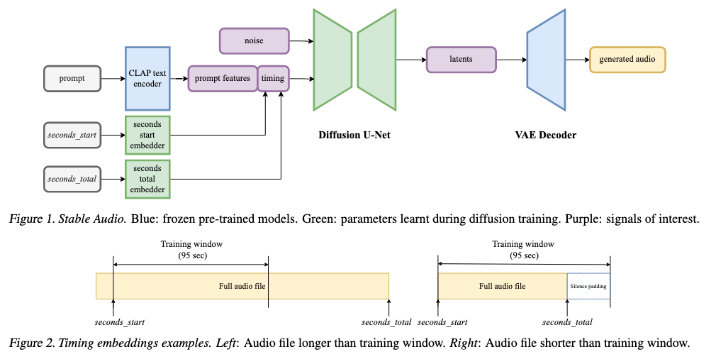
3.2 Conditioning: Telling the Model What and How Long to Generate
To steer the model’s output, Stable Audio uses two kinds of conditioning signals: Text prompts and Timing embeddings.
📝 Text Encoder: CLAP to the Rescue
- The team uses a CLAP-based encoder — a contrastive language-audio pretraining model.
- It’s trained from scratch on their own dataset (not just the open-source CLAP).
- Instead of using the final layer (as many do), they use the next-to-last hidden layer, inspired by practices in visual-language models like CLIP and Stable Diffusion. This layer tends to preserve more useful context for generation.
- These text embeddings are passed to the U-Net via cross-attention layers.
Why not T5 or MuLan?
- Because CLAP learns audio-text relationships, making it more suitable for describing sound-rich prompts like “ambient rainforest with tribal drums”.
🕒 Timing Embeddings: Fine-Grained Control Over Duration
Stable Audio pioneers the idea of timing-aware diffusion for audio. Here’s how it works:
- From each training clip, two timing values are recorded:
- seconds_start: Where the chunk begins in the original audio
- seconds_total: The full duration of the original audio
📌 Example:
If you sample a 95-sec chunk from a 180-sec track starting at 14s:
- seconds_start = 14
- seconds_total = 180
These are then turned into learned per-second embeddings, and concatenated with the text features. They are fed into the model via cross-attention.
During inference, you can set:
- seconds_start = 0, seconds_total = 30 to get a 30-sec output
- The remaining time (e.g. 65 sec) is padded with silence in the latent space
💡 Why this matters:
- Supports variable-length generation
- Eliminates hardcoded clip lengths
- Allows users to request specific durations
And yes — silence padding is easy to trim afterward.
3.3 Diffusion Model: The Brain Behind the Music
The actual denoising (i.e. generation) happens in a U-Net diffusion model with 907M parameters. It’s inspired by Moûsai and tailored to scale up with long latents.
U-Net Design
- 4 Levels of encoder-decoder blocks
- Downsampling factors: 1×, 2×, 2×, 4× (i.e. progressively compress along length)
- Channel sizes: 1024, 1024, 1024, 1280
- Skip connections between encoder and decoder layers maintain resolution-specific features
Inside Each Block
- 2 Conv residual layers
- 1 to 3 attention layers:
- Self-attention
- Cross-attention for text + timing
- Bottleneck block between encoder and decoder with 1280 channels
- Fast attention kernels (from Dao et al., 2022) to optimize memory and speed
Conditioning Layers
- FiLM (Feature-wise Linear Modulation) layers inject timestep noise level info (i.e. how noisy the latent currently is)
- Cross-attention layers inject text + timing information
🎞️ FiLM (Feature‑wise Linear Modulation)
FiLM, introduced by Perez et al., 2017, lets a neural network adapt its internal features using an external input — e.g. text, labels, or (for diffusion models) the timestep.
The Core Idea
Given a feature map \(F \in \mathbb{R}^{C \times H \times W}\) and a conditioning vector \(c\), FiLM learns per‑channel scale & shift:
$$\text{FiLM}(F;\gamma,\beta) \;=\; \gamma(c)\,F \;+\; \beta(c)$$
- \(\gamma(c)\) — MLP outputs channel‑wise scales
- \(\beta(c)\) — MLP outputs channel‑wise shifts
In Diffusion Models
The timestep \(t\) is embedded, passed through MLPs to get \(\gamma(t)\) and \(\beta(t)\), then applied:
$$\text{FiLM}(x) = \gamma(t)\,x + \beta(t)$$
Effect: The network “knows” how noisy the input is and modulates its features accordingly — gentle cleaning early on, fine‑grain denoising later.
Why Not Just Concatenate the Timestep?
- More expressive — can amplify or suppress specific channels per step.
- Modular — injects conditioning exactly where needed.
- Widely adopted — Imagen, Muse, Latent Diffusion, etc.
3.4 Inference: Fast, Controlled Sampling
During inference, Stable Audio uses:
- DPMSolver++: A fast, high-quality diffusion sampler
- Classifier-free guidance (CFG): Amplifies the conditioning signal (scale = 6)
- 100 diffusion steps: Chosen as a balance between speed and audio quality (details in Appendix A)
💡 The final audio:
- Can be up to 95 sec
- Will contain silence after your specified seconds_total
-
Silence can be trimmed post-hoc — works reliably due to strong timing embeddings (as validated in Section 6.3)
⚡ DPMSolver++ (Fast Diffusion Sampler)
DPMSolver++ (Denoising Probabilistic Matching Solver++) is a fast & accurate sampler for diffusion models, introduced by Lu et al., 2022.
Why Sampling Matters
- Diffusion starts with pure noise and denoises over
Tsteps. - Each step = one forward pass → speed bottleneck.
- Vanilla DDPM needs 1000+ steps; DPMSolver++ can deliver high‑quality samples in ≈ 15 – 100 steps.
What Makes DPMSolver++ Special?
- ODE‑based formulation — models the true probabilistic path.
- Higher‑order solvers — 2nd / 3rd‑order integration for accuracy at large step sizes.
- Explicit update rules — maintain the diffusion process’s statistical properties.
- Outperforms DDIM, PLMS, etc., at similar step counts.
Practical Upshot
Swap in DPMSolver++ → ~10× faster inference with negligible (or no) loss in perceptual quality.
4 Training
4.1 Dataset: The Backbone
Stable Audio is trained on a massive dataset of 806,284 audio files totaling 19,500 hours from AudioSparx, a stock music provider.
Dataset Breakdown:
- Music: 66% of the files (or 94% of total audio hours)
- Sound effects: 25% of files (5% of hours)
- Instrument stems: 9% of files (1% of hours)
Each file comes with rich text metadata, including:
- Descriptions (e.g., “epic orchestral cinematic rise”)
- BPM
- Genre
- Mood
- Instrument labels
📌 The dataset is public for consultation — a win for transparency and reproducibility.
4.2 Training the VAE: Compressing Without Losing Musicality
The VAE (used to compress audio into latents) was trained on 16 A100 GPUs using automatic mixed precision (AMP) for 1.1 million steps.
AMP
What is Automatic Mixed Precision (AMP)?
AMP is a technique that allows deep learning models to use both 16-bit (float16) and 32-bit (float32) floating-point numbers during training — automatically.
Traditionally, models are trained in float32 precision (a.k.a. FP32), which is precise but:
- Slower to compute
- Uses more GPU memory
With AMP:
- Some operations (like matrix multiplications) are done in float16 (FP16) — faster and smaller
- Others (like loss computation or gradient updates) stay in float32 — more stable and accurate
The “automatic” part means you don’t need to manually specify which ops use which precision — your framework (like PyTorch or TensorFlow) figures it out for you.
Pros:
- Faster training: On GPUs like NVIDIA A100s or V100s, FP16 operations are 2–8× faster than FP32.
- Lower memory usage: FP16 uses half the memory, so you can train larger models or bigger batches.
- Same or similar accuracy: Thanks to dynamic loss scaling and smart casting, AMP usually retains almost all the performance of full-precision training.
Challenges:
- FP16 has a narrower range of values (can underflow or overflow), which may cause instability if used naively.
- That’s why AMP keeps sensitive operations in FP32, like:
- Loss calculation
- Gradients accumulation
- Batch norm updates
Strategy
- Phase 1: Train both encoder and decoder for 460,000 steps.
- Phase 2: Freeze the encoder, fine-tune the decoder for 640,000 more steps — this improves reconstruction fidelity without changing latent space.
Loss Functions
They used a carefully crafted loss mix focused on stereo audio fidelity:
| Loss Type | Description |
|---|---|
| 🎧 STFT Loss | Multi-resolution sum-and-difference STFT (to ensure left/right stereo correctness), applied after A-weighting to match human hearing |
| 🧠 Adversarial Loss | From a multi-scale STFT discriminator with patch-based hinge loss (encourages realism) |
| 🧪 Feature Matching | Matches internal features of real vs generated audio |
| 📉 KL Loss | Keeps the latent space well-behaved |
Window sizes for STFT:
[2048, 1024, 512, 256, 128, 64, 32] (for reconstruction) and
[2048, 1024, 512, 256, 128] (for adversarial discriminator)
Loss weights:
- STFT loss: 1.0
- Adversarial: 0.1
- Feature matching: 5.0
- KL divergence: 1e-4
This blend ensures high fidelity, structure, and stereo realism in reconstruction.
4.3 Training the Text Encoder: CLAP, from Scratch
They trained their CLAP model (contrastive language-audio pretraining) from scratch on the same dataset.
Setup:
- 100 epochs
- Batch size: 6,144
- Hardware: 64 A100 GPUs
- Uses the original CLAP configuration:
- RoBERTa-based text encoder (110M parameters)
- HTSAT-based audio encoder (31M parameters)
- Loss: Language-audio contrastive loss
🎯 Result: A multimodal text encoder deeply aligned with their dataset — outperforming open-source CLAP or T5 in text-to-audio alignment.
4.4 Training the Diffusion Model
Once the VAE and CLAP were ready, they trained the latent diffusion model.
Setup:
- 640,000 steps
- 64 A100 GPUs
- Batch size: 256
- Exponential moving average (EMA) of model weights
- AMP enabled for memory-efficient training
Audio Preparation:
- Resample to 44.1kHz
- Slice to exactly 95.1 seconds (4,194,304 samples)
- Crop long files from random point
- Pad short ones with silence
Objective:
- v-objective (Salimans & Ho, 2022): A more stable variant of denoising objective
- Cosine noise schedule (smoothly decays noise over time)
- Continuous timestep sampling
💡 Dropout (10%) applied to the conditioning inputs → this enables classifier-free guidance during inference (a trick borrowed from image models).
Note: Text encoder was frozen during diffusion training — so only the U-Net learns how to use its features.
4.5 Prompt Preparation: How Text Prompts Were Created
Each audio file had rich metadata, but not all of it was equally useful all the time.
So they used dynamic prompt construction during training:
- Create synthetic natural-language prompts by randomly sampling metadata fields.
- Two styles:
-
Structured:
Instruments: Guitar, Drums | Moods: Uplifting, Energetic -
Free-form:
Guitar, Drums, Bass Guitar, Uplifting, Energetic
-
- Shuffle the items to prevent the model from overfitting to order.
This makes the model robust — it can understand both natural text and structured metadata during inference.
5 Methodology
Generating high-quality, realistic, and text-aligned music or sound effects is already hard — but measuring how good that generation is? Even harder. Especially when you’re dealing with long-form, stereo, high-fidelity audio.
5.1 Quantitative Metrics
1. FDOpenL3 — Realism
The Fréchet Distance (FD) is a go-to metric in generative modeling. It checks how similar the statistics (mean, covariance) of generated content are to real content — in a learned feature space.
Stable Audio’s Twist
- Instead of projecting audio into VGGish features (which are 16kHz and mono), they use OpenL3, which handles up to 48kHz and stereo.
- Stereo-aware: They feed left and right channels separately, get OpenL3 features for each, and concatenate.
- For mono baselines, they simply copy the features to both sides.
✅ FDOpenL3 evaluates:
- Realism of generated long-form
- Full-band stereo audio at 44.1kHz
2. KLPaSST — Semantic Alignment
How much do the generated sounds semantically match their reference content?
They use:
- PaSST: A strong audio tagging model trained on AudioSet
- Compute the KL divergence between the label probabilities of generated vs real audio
Stable Audio’s Twist:
- PaSST only supports up to 32kHz, so they resample from 44.1kHz
- Audio is segmented into overlapping chunks, logits are averaged, and softmax is applied
✅ KLPaSST captures:
- Tag-level alignment (e.g., “rock”, “violin”, “clapping”)
- Works for variable-length audio, not just 10-second snippets
3. CLAPscore — Prompt Adherence
CLAP (Contrastive Language-Audio Pretraining) is used to measure how well the generated audio matches the text prompt.
Stable Audio’s Twist:
- Instead of using just a single 10s crop (like prior works), they use feature fusion:
- A global downsampled version of the full audio
- Plus 3 random 10s crops from beginning, middle, and end
- This fused signal is encoded using CLAP-LAION (trained on 48kHz)
- Both the text and audio embeddings are compared via cosine similarity
✅ CLAPscore tests:
- How well long-form stereo audio adheres to the prompt
- Works across full audio — intro, middle, and end
5.2 Qualitative Metrics
Beyond math and embeddings — what do humans think?
Human evaluation criteria:
| Metric | Description |
|---|---|
| 🎧 Audio quality | Is it high-fidelity or noisy/low-res? |
| ✍️ Text alignment | Does the sound match the prompt? |
| 🎵 Musicality | Are melodies/harmonies coherent? |
| 🔊 Stereo correctness | Does the left/right channel sound appropriate? |
| 🏗️ Musical structure | Does the music have an intro, middle, and outro? |
Ratings Collected:
- Audio quality, Text alignment, Musicality: Rated on a 0–4 scale (bad → excellent)
- Stereo correctness & Musical structure: Binary (Yes/No)
Special rules:
- Musicality/structure: Only evaluated for music
- Stereo correctness: Only for stereo signals
- Non-music: Only quality, alignment, stereo correctness
Evaluations were run using webMUSHRA, a standardized perceptual testing framework.
5.3 Evaluation Data
They used two popular text-audio benchmarks:
MusicCaps
- 5,521 music clips with 1 text caption each
- YouTube-based, mostly stereo
- Only 10-second clips — so Stable Audio generated longer clips (up to 95 sec)
AudioCaps
- 979 clips with 4,875 total captions
- Also YouTube-based, mostly stereo
- Focuses on environmental sounds and effects
Challenge:
- Captions only describe the first 10 seconds, so reference comparisons are limited.
- Stable Audio still generates longer audio — showing its ability to go beyond what’s seen during training.
5.4 Baselines
Some top models (e.g., Moûsai, JEN-1) weren’t comparable due to lack of open-source weights.
So they compared against open-source SOTA:
| Model | Type | Notes |
|---|---|---|
| AudioLDM2 | Latent Diffusion | 48kHz mono and 16kHz variants |
| MusicGen | Autoregressive | Small and large models, stereo version available |
| AudioGen | Autoregressive | Medium-sized, for sound effects |
Notes:
- AudioLDM2 = best non-autoregressive open baseline
- MusicGen-stereo = best autoregressive stereo baseline
- MusicGen doesn’t model vocals, so vocal prompts were filtered in some tests
6 Experiments
6.1. How Good Is the Autoencoder?
To test how much audio quality is lost in the compression and decompression process (via the VAE), the authors:
- Passed real training audio through the encoder → decoder pipeline
- Compared the output to the original using FDOpenL3
🧠 Result: The autoencoded audio showed slightly worse FD scores than the original, but the degradation was minimal. Informal listening confirmed the fidelity is transparent — meaning humans barely notice the difference.
6.2. Which Text Encoder Works Best?
They tested:
- CLAP-LAION (open-source)
- CLAPours (trained from scratch on their dataset)
- T5 (text-only encoder)
Each version was frozen during training, and the base model was trained for 350K steps.
🧠 Result: All performed comparably, but CLAPours slightly outperformed the others. Since it was trained on the same dataset as the diffusion model, it offered better vocabulary alignment and semantic grounding.
✔️ Final Choice: CLAPours — for consistency and performance.
6.3. How Accurate Is the Timing Conditioning?
They tested if the model could:
- Generate audio of exactly the length requested via timing embeddings.
- Do this across many durations (from short to long).
They used a simple energy-based silence detector to find where the real content ended in the generated 95s audio window.
🧠 Result:
- The model closely follows the expected duration
- Most accurate at short (≤30s) and long (≥70s) durations
- Some variability around 40–60 seconds, likely due to fewer training examples of this length
- Some misreadings caused by limitations of the silence detection method
6.4. How Does It Compare to State-of-the-Art?
Benchmarks are shown in Tables 1–3 (not included here), comparing Stable Audio against:
- AudioLDM2
- MusicGen (small, large, stereo)
- AudioGen
Key Observations:
- Best in audio quality and text alignment on MusicCaps
- Slightly weaker on AudioCaps for text alignment, possibly due to fewer sound effects in its training set
- Competitive in musicality and musical structure
- Good at stereo rendering for music but weaker on stereo correctness for effects — possibly because some prompts don’t require spatial diversity
- Importantly, it’s the only model consistently capable of generating intro → development → outro — real musical structure, not just loops
6.5. How Fast Is It?
They benchmarked inference time on a single A100 GPU (batch size = 1).
🧠 Result:
- Much faster than autoregressive models (e.g., MusicGen, AudioGen)
- Faster than AudioLDM2, even when generating higher-quality audio (44.1kHz stereo vs. 16kHz or mono)
- Particularly faster than AudioLDM2-48kHz, which works at a similar bandwidth but takes longer
✅ Latent diffusion + optimized architecture + DPMSolver++ = speed with quality
Section 7: Conclusions
Stable Audio proves that it’s possible to build a system that is:
- 🎵 Flexible (supports music and sound effects)
- ⏱️ Fast (generates up to 95s in just 8s)
- 🎧 High-fidelity (44.1kHz stereo)
- 🧠 Controllable (via text + timing conditioning)
- 🧪 Well-evaluated (with new long-form-aware metrics)
It pushes the frontier in multiple areas:
- One of the first systems to consistently generate structured music
- Among the few to generate stereo sound effects
- Introduces new metrics for evaluating long-form, full-band, stereo generation
- Outperforms or competes with state-of-the-art in multiple benchmark