Noise2Music: Text-conditioned Music Generation with Diffusion Models
1 Summary
Goal: Turn a plain‑language prompt (“a slow lo‑fi guitar ballad for a rainy afternoon”) into a 30‑second, 24 kHz stereo clip.
Approach – Train several diffusion models that run one after another (a cascade). The early stages sketch a coarse spectral “layout”; later stages fill in detail so the final waveform sounds clean and full‑bandwidth.
Why a cascade of diffusion models?
A single diffusion model that jumps straight from noise→high‑fidelity audio would need huge compute and might blur fine structure. Splitting the job lets each stage specialise:
- Generator – predicts a low‑resolution latent audio representation conditioned on the text.
- Cascader(s) – progressively upsample and refine that latent into the final waveform (16kHz), optionally re‑checking the text each step.
- Super‑resolution: A final superresolution cascader is used to generate the 24kHz audio from the 16kHz waveform.
- All models are based on 1D U-Nets
Two options for the intermediate representation:
- Spectrogram (log-mel)
- Audio with lower fidelity (3.2kHz waveform)
Results:
- Generated audio faithfully reflect key elements of the text prompt such as genre, tempo, instruments, mood, and era.
- Ground finegrained semantics of the prompt.
Data
Text labels for the audio are generated by employing a pair of pretrained deep models:
- Use a large language model to generate a large set of generic music descriptive sentences as caption candidates;
- Pre-trained music-text joint embedding model is used to score each unlabeled music clip against all the caption candidates and select the captions with the highest similarity score as pseudo labels for the audio clip.
- Annotate O(150K) hours of audio sources
2 Related Works
- Over the past five years, the recipe for dramatic jumps in sample quality has been simple: bigger datasets + bigger models.
How models ingest “what I want”
- Fixed, human‑interpretable vocabularies
- Jukebox encodes each clip as one of ~8 k artist/genre labels extracted from its metadata.
- Mubert maps a user prompt onto a hand‑curated tag set (e.g., “chill”, “EDM”, “focus‑music”).
- Pros: Easy to reason about.
- Cons: Can’t express “dreamy underwater lo‑fi.”
- Free‑form natural language embeddings
- AudioGen, MusicLM and Noise2Music feed the raw prompt through a frozen text encoder (e.g., MuLan or a language‑model encoder).
- Pros: Unlimited expressiveness; prompts can describe mood, setting, instrumentation, era, etc.
- Cons: The mapping from prose → sound is learned, not predefined, so training data must be rich.
3 Methods
3.1 Diffusion models in a nutshell
Diffusion models turn pure noise into a data sample by iterative denoising. Two ingredients go in at each step:
- Conditioning signal \(c\) – here, the text‑prompt embedding.
- Noisy input \(x_t\) – a corruption of the target waveform at “time” t, where t ∈ [0, 1]. Noise magnitude is set by a schedule \(σ_t\).
During training the model \(θ\) learns to predict the exact noise vector \(ϵ\) that was added:
\[\mathcal{L} \;=\; \mathbb{E}_{x,c,\epsilon,t}\!\bigl[ w_t \,\lVert \theta(x_t, c, t) \;-\; \epsilon \rVert^2 \bigr],\tag{1}\]where \(w_t\) is a hand‑chosen weight (details below).
Choosing the loss weight \(w_t\):
| Option | Rationale |
|---|---|
| Simplified (\(w_t\) = 1) | Easiest to implement, works well for many tasks. |
| Sigma‑scaled (\(w_t\) = \(σ_t^2\)) | Emphasises accuracy at late (cleaner) timesteps. |
Noise‑schedule variants
| Schedule | Shape | Typical use‑case |
|---|---|---|
| Linear | \(σ_t\) grows linearly with t | Classic DDPM baseline. |
| Cosine | Slower rise near t = 0, faster near t = 1 | Often yields crisper samples with fewer steps. |
Sampling: knobs you can turn
At inference we start with pure noise at t = 1 and march back to t = 0 (“ancestral” or DDPM sampling). Two important dials:
| Dial | Symbol | Effect |
|---|---|---|
| Stochasticity | \(γ ∈ {0, 1}\) | \(γ\) = 0 gives deterministic DDIM‑like steps; γ = 1 keeps full randomness. |
| Denoising Step schedule | \({t_0 … t_n}\) | Any partition of [0, 1] works—e.g., 50, 100, or 1 000 steps. |
\(γ\) : Sets how much fresh Gaussian noise is re‑added at every reverse‑diffusion step.
Classifier‑free guidance (CFG)
To better align outputs with the text prompt, the authors adopt CFG:
- During training: Randomly drop the prompt for a subset of samples → model learns both conditional \(θ(x_t, c)\) and unconditional \(θ(x_t, ·)\).
- During sampling: Blend the two predictions:
Larger w tightens adherence to the prompt but risks clipping; the paper counters this with dynamic clipping that scales intermediate values to a safe range.
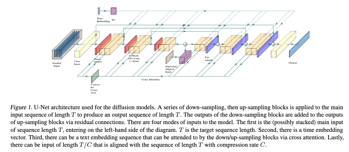
3.2 Model Architecture — “Efficient U‑Net 1‑D”
Backbone. A 1‑D adaptation of the Efficient U‑Net:
- Down / Up blocks: They shrink the audio signal to a smaller size (down‑sampling) or stretch it back up (up‑sampling). Inside each block, the model mixes basic convolutions with attention layers to learn both local details and long‑range relationships.
- Combine layer: The combine layer enables a single vector to interact with a sequence of vectors, where the single vector is used to produce a channel-wise scaling and bias.
- A single vector (like the “time‑step” embedding) can turn channels up or down and add a bias, letting the model adapt its behaviour at each diffusion step.
- More on Combine Layers
- Inputs
- Feature map A sequence of vectors coming from the convolution/attention stack. Shape: (length, channels).
- Condition vector z A single 1‑D vector (e.g., the diffusion‑time embedding, or any global conditioning info). Shape: (channels).
- Learned transform
- The layer passes \(z\) through two tiny neural nets (often single linear layers) to produce
- Scale s - one value per channel
- Bias b - one value per channel
- The layer passes \(z\) through two tiny neural nets (often single linear layers) to produce
- Channel‑wise modulation
-
For every position \(i\) in the sequence and every channel c
\[\text{output}_{i,c}=s_c \times \text{feature}_{i,c}+b_c\] -
This is just an affine transform (scale + shift), but the scales/biases change with \(z\).
-
- Why it matters
- Lets a global signal (time step, overall prompt embedding, etc.) instantly tweak the local activations without extra convolutions.
- Makes conditioning cheap and expressive—similar in spirit to FiLM layers used in vision models.
- Inputs
Four conditioning routes
- Noise input \(x_t\) (always left‑most in the stack).
- Diffusion‑time embedding fed via Combine layers.
- Text prompt sequence enters through cross‑attention.
-
Low‑resolution audio or spectrogram (aligned) can be injected at the U‑Net bottleneck.
3.3 Cascaded Diffusion: three‑stage pipeline
Noise2Music follows the Generator → Cascader → Super‑Resolution recipe.
3.3.1 Waveform Model
Generator
- Input: Text prompt
- A sequence of vectors derived from the text input is produced and fed into the network as a cross-attention sequence
- Outputs: 3.2 kHz waveform
Cascader
- Inputs: Conditioned on both the text prompt and the low-fidelity audio generated by the generator model based on the text prompt.
- Outputs: 16 kHz waveform
- Method:
- The text conditioning takes place via cross attention.
- Low-fidelity audio is upsampled and stacked with \(x_t\) and fed into the model.
- The upsampling is done by applying fast Fourier transform (FFT) to the low-fi audio sequence and then applying inverse FFT to obtain the high-fi audio from the low-fi Fourier coefficients.
3.3.2 Spectrogram Model
Generator
- Outputs: 80‑×‑100 fps log‑mel spectrogram (80 channels and a frequency of 100 features per second)
- Pixel values of the log-mel spectrogram are normalized to lie within [−1, 1]
Vocoder
- Output: 16kHz audio that is conditioned only on the spectrogram
3.3.3 SUPER-RESOLUTION CASCADER
- Generate 24kHz audio from the 16kHz waveform produced by either model.
- The 16kHz audio is up-sampled and stacked with \(x_t\) as input to the model.
- Text conditioning is not used for this model.
3.4 Text Understanding
T5 encoder:
- Prompt’s token‑level embeddings without pooling are feed into cross‑attention layers throughout the U‑Net
3.5 Pseudo‑Labeling for Music Data [DATA Creation]
3.5.1 Why pseudo‑labels are needed
- High‑quality music + free‑form caption pairs are rare.
- Without them, a text‑to‑music model can’t learn subtle descriptors like “laid‑back highway‑driving synthwave.”
- Solution: auto‑generate rich captions for millions of unlabeled tracks instead of hand‑annotating them.
3.5.2 Models Used
MuLan: A contrastive model with audio and text encoders that share an embedding space.
- Lets you measure “text–audio similarity” with cosine distance (zero‑shot classification).
LaMDA: LLM trained for dialogue.
- Used here to write human‑style music descriptions.
3.5.3 Building three caption vocabularies
| Name | Size | How it’s made | Purpose / style |
|---|---|---|---|
| LaMDA‑LF | 4 M long‑form sentences | Prompt LaMDA with title + artist of 150 000 popular songs → clean & deduplicate. | Conversational, user‑prompt‑like prose. |
| Rater‑LF | 35 333 sentences | Split 10 028 expert captions from MusicCaps into single sentences. | Human‑written, descriptive. |
| Rater‑SF | 23 906 short tags | Collect all short aspect tags from the same raters (mood, genre, instrument, etc.). | Compact, label‑like keywords. |

3.5.4 Assigning captions to an unlabeled clip
- Segment clip into 10‑s windows → feed each window to MuLan’s audio encoder.
- Average those embeddings → one vector per clip.
- Encode every caption in the vocabularies with MuLan’s text encoder.
- Retrieve the K = 10 closest captions (cosine similarity).
- Sample K′ = 3 of those 10, with probability \(∝\) 1 / global_frequency (rare captions get a boost).
- Balances the label distribution and increases diversity.
- Store the selected captions as pseudo‑labels for that clip.
Net effect: each 30‑s clip can receive up to 12 pseudo‑labels (3 from LaMDA‑LF, 3 from Rater‑LF, 6 from Rater‑SF) in addition to any inherent metadata.
3.5.5 Warm‑up experiment: MuLaMCap
- Source: AudioSet’s music subtree — 388 262 train clips + 4 497 test clips (each 10 s).
- Labels per clip: 3 × 3 + 3 × 3 + 6 × 6.
- Purpose: sanity‑check the pipeline before scaling to millions of tracks.
3.6 Training‑Data Mining at Scale [DATA]
- Raw audio pool
- 6.8 million full‑length music tracks are collected.
- Each track is chopped into six non‑overlapping 30‑second clips → ~340 000 hours total.
- Sample rates
- 24 kHz clips train the super‑resolution stage (it must output 24 kHz).
- 16 kHz versions of the same clips train every other model stage (saves compute).
-
Text labels attached to every clip
Label source Count per clip What it adds Song title 1 “Hotel California” Named‑entity tags variable Genre, artist, instrument, year, etc. LaMDA‑LF pseudo‑labels 3 Rich sentences like “slow acoustic ballad for a summer evening.” Rater‑SF pseudo‑labels 6 Compact tags such as “laid‑back,” “highway‑driving,” “lo‑fi beats.” Why skip Rater‑LF?
- Those captions appear in the MusicCaps evaluation set; excluding them avoids train‑test leakage.
- Why mix “objective” and “subjective” labels?
- Objective tags (genre, artist) nail down obvious metadata.
- Pseudo‑labels add nuances—mood, activity, fine‑grained compositional hints.
- Together they give the model both facts and feelings to learn from.
- Quality anchor inside the noisy sea
- The authors add ≈ 300 hours of internally curated, attribution‑free tracks.
- Each track’s rich metadata is concatenated into a single prompt string.
- Acts as a clean, high‑signal subset to stabilize training.
Net result: a gigantic, diverse corpus where every 30‑s clip carries 10 + text descriptors that range from “objective metadata” to “subjective vibes,” providing the breadth of supervision a text‑to‑music diffusion model needs.
4 Experiments and Results
4.1 Model training details
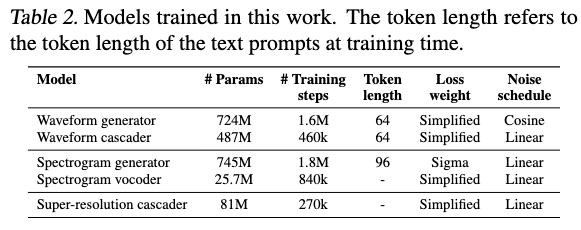
Models trained: 4 separate 1‑D U‑Nets
- Waveform Generator (3.2 kHz)
- Waveform Cascader (16 kHz)
- Spectrogram Generator (80 × 100 fps log‑mel)
- Spectrogram Vocoder (16 kHz)
Final 24 kHz “super‑res” U‑Net is a light extension of the cascader.
Loss Weighting
- σ²‑weighted MSE for spectrogram generator (critical for convergence)
- Weighs the loss more heavily on the “back end” (late or cleaner timesteps) of the denoising schedule.
- Either σ² or constant 1 for others
Note: All the models, with the exception of the vocoder, are trained on audio-text pairs, while the vocoder is only trained on audio.
Text batch per clip
- Long‑form descriptions (3 items) comes from LaMDA‑LF vocabulary and stored as three different strings.
- Short tags and metadata - mashed together, then chopped to size
- All of them are concatenated into one line
- If this string exceeds the token limit fixed in Table 2 (say 64 tokens), it is split into equal‑length chunks so that each chunk fits the limit.
- Every chunk counts as an additional candidate caption.
- Total = 3 long sentences + 1 – 2 short chunks (depending on length).
During training the loader randomly picks one element from that list and feeds it to the U‑Net as the text conditioning for this audio example.
- So across epochs the network sees the same audio paired sometimes with a rich prose description, other times with a terse tag bundle—helping it learn both broad language and concise labels.
More Details
Optimizer:
- Adam, \(β_1\) = 0.9, \(β_2\) = 0.999
LR schedule:
- Cosine LR Scheduler, Max LR: 1 × 10⁻⁴
- End Point: Step 2.5 M, Warm-Up steps: 10 k
Exponential Moving Average (EMA)
Individual parameter updates from each mini‑batch are noisy. Averaging them over time gives a smoother, typically better‑generalising set of weights for inference.
\[\theta_{t} = (1-\alpha)\,\theta_{t-1} + \alpha\,\theta_{t}\]- Decay factor d = 1 − α , d = 0.9999 and used at inference time.
- Keep a second weight copy while training (EMA)
- Snapshot those EMA weights to disk
- At inference time → Load only the EMA copy (ignore the noisy “online” weights).
- Why this works
- Reduces training‑loss noise.
- EMA weights have seen every past setting of the model, so outliers cancel out.
- Empirically they yield crisper audio and fewer artifacts, especially for diffusion and GAN‑style generators.
Batch Size
- 4096 for Super-res cascader (since its lightweight)
- 2048 for rest
CFG During Training
- Hide prompt for 10 % of samples (cross‑attention outputs zeroed)
- Teaches model to handle both conditional and unconditional cases, enabling CFG at inference.
Sequence length seen by each model
- Generators: full 30 s clip
- Cascader & vocoder: random 3–4 s windows
- Cascader/vocoder don’t use self‑attention → can train on snippets, saving memory.
Data augmentations (for cascader & vocoder)
Randomly corrupt the conditioning low-fidelity audio or the spectrogram input by applying diffusion noise
- Random diffusion time is chosen within [0, \(t_{max}\)] and applied to the intermediate representation of the audio, i.e., the upsampled low-fi audio or the spectrogram.
- Cascader \(t_{max}\): 0.5
- Vocoder and super-res \(t_{max}\): 1.0
Blur Augmentation of conditioning input
- For the cascader model, a 1D blur kernel of size 10 is used with a Gaussian blur kernel whose standard deviation ranges from 0.1 to 5.0.
- For the vocoder model, a 2D 5x5 blur kernel is applied with the standard deviation ranging from 0.2 to 1.0.
4.2 Model inference and serving
4.2.1 Model Inference
- Three knobs you can turn
- Denoising schedule – how you spread the diffusion steps along time t∈[0, 1].
- Stochasticity γ – 0 = deterministic (DDIM‑style), 1 = full randomness (DDPM‑style).
- CFG scale w – how strongly the result must obey the text prompt (larger w → tighter match, but riskier artefacts).
- What “denoising schedule” really means
- Imagine you have N small time jumps \(δ₁…δ_N\) that must add up to 1.
- Front‑heavy: many tiny steps right at the start (when audio is still noisy).
- Uniform: equal spacing throughout.
- Back‑heavy: more steps near the end (when audio is already fairly clean).
- Given a fixed budget of steps, choosing where to spend them is a trade‑off between global structure (benefits from early steps) and fine detail (benefits from late steps).
- Hyper‑parameter sets actually used
- Each of the four U‑Nets (generator, cascader, spectrogram generator, vocoder) gets its own trio of settings (schedule type, γ, CFG scale).
- Those exact numbers live in Table 3 of the paper; the principle is the same: early models lean slightly “front‑heavy” and higher γ for creativity, while later refiners go “back‑heavy” and lower γ for polish.


4.3 Evaluation
- Parameter Selection for the Models
- Team used a handful of private “dev prompts,” listened, and chose the versions that subjectively sounded best within their compute budget.
- All metrics are computed on the 16 kHz outputs straight from the cascader/vocoder — the 24 kHz super-resolution stage is skipped during evaluation.
- 4.3.2 Evaluation Metrics
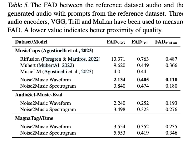
- Fréchet Audio Distance (FAD): same idea as FID for images. Three encoders give three flavours:
- VGGish → general sonic quality.
- Trill → vocal-centric quality.
- MuLan audio encoder → high-level musical semantics.
- MuLan similarity: cosine similarity in the MuLan embedding space. Used two ways:
- Text ↔ generated audio (how well the clip matches its prompt).
- Ground-truth audio ↔ generated audio.
- Randomly shuffled pairs give a “chance level” baseline.
- Fréchet Audio Distance (FAD): same idea as FID for images. Three encoders give three flavours:
- Evaluation datasets
- MagnaTagATune (MTAT) — 21 638 clips with up to 188 tag labels concatenated into a single prompt; model generates a full 29-s clip.
- AudioSet-Music-Eval — 1 482 ten-second clips; tags concatenated; model generates 30 s, middle 10 s are scored.
- MusicCaps — 5.5 K ten-second clips with rater-written free-form captions; model generates 30 s, middle 10 s are scored.
4.4 Results
4.5 Inference-time ablations
- Classifier-free guidance (CFG) scale
- Sweet spot around 5–10; beyond that, FAD rises and audio gets over-compressed or distorted.
- Generator’s CFG weight matters more than its denoising schedule; for the cascader it’s the opposite.
- Denoising schedule shape
- Cascader is very sensitive: front-heavy schedules hurt quality; back-heavy gives best FAD & similarity.
- Generator is less sensitive; uniform vs. mildly front-heavy are both acceptable.
- Step count vs. quality (cost curve)
- More steps in the cascader/vocoder nearly always help; extra steps in the generator give diminishing returns after a point.
- Plot shows the elbow where doubling steps adds little perceptual gain — useful for setting latency targets.
5 More
Spectrogram vs. waveform cascades
- Spectrogram path
- Much cheaper to train and serve because the input sequence is short.
- Naturally keeps high‑frequency detail that a 3 kHz low‑fi waveform cannot contain.
- Down‑side: intermediate representations are hard for engineers to interpret/debug.
- Waveform path
- Every intermediate output is an actual audio snippet, which makes debugging and hyper‑parameter tuning easier.
- Training/serving is costlier and sequence length limits scalability to very long clips.
Open research directions
- Better interpretability and controllability.
- Stronger text–audio alignment (fewer “off‑prompt” generations).
- Lower training and inference cost.
- Longer outputs, plus tasks such as music in‑painting or style transfer—analogous to image editing with diffusion “paint‑over” techniques.