Denoising Diffusion Probabilistic Models

Ho, Jonathan, Ajay Jain, and Pieter Abbeel. “Denoising Diffusion Probabilistic Models.” arXiv:2006.11239. Preprint, arXiv, December 16, 2020. https://doi.org/10.48550/arXiv.2006.11239.

Code

Table of Contents

• Abstract
• Diffusion Models
  • The Forward Process (Data → Noise)
  • The Reverse Process (Noise → Data)
• Training Objective
  • Variational Lower Bound Loss
  • Expanding the Variational Bound
  • Rewriting the Loss
  • Parameterisation Trick
  • The Simplified Objective
• Training Algorithm
  • Connection to Score Matching
  • More
• Experiments

Abstract

• High quality image synthesis results using diffusion probabilistic models.
  • Latent‑variable model – The model assumes there’s an unobserved variable z that, after some transformation, produces your image x.
• Trained on Weighted variational bound designed according to a novel connection between diffusion probabilistic models and denoising score matching with Langevin dynamics.

Diffusion Models

We use Diffusion probabilist model (aka Diffusion Models). They are a class of generative models that learn to create high-quality samples by reversing a gradual corruption process.

More Details on Diffusion models → diffusion-models.html

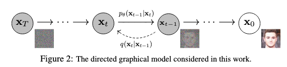
The Forward Process (Data → Noise)

Markov chain that gradually adds Gaussian noise to the data according to a variance schedule: \(β_1, . . . , β_T\). It gradually corrupts the original data by adding Gaussian noise:

\[q(x_{1:T}|x_0) = ∏^T_{t=1} q(x_t|x_{t-1})\] \[q(x_t|x_{t-1}) = N(x_t; \sqrt{(1-β_t)}x_{t-1}, β_tI)\]

Key aspects:

• \(x_0\): Original clean data
• \(x_1, x_2, ..., x_t\): Progressively noisier versions
• \(β_t\): Variance schedule controlling how much noise is added at each step
• This process is fixed and doesn’t require learning

The Reverse Process (Noise → Data)

The reverse process learns to undo the forward corruption:

\[p_θ(x_{0:T}) = p(x_T) ∏_{t=1}^T p_θ(x_{t-1}|x_t)\] \[p_\theta(x_{t-1} \mid x_t) \;=\; \mathcal{N}\!\Bigl( x_{t-1} \;;\; \mu_\theta(x_t, t), \;\Sigma_\theta(x_t, t)\Bigr)\]

Key aspects:

• Starts from pure noise: \(p(x_T) = N(x_T; 0, I)\)
• Each step is a learned Gaussian transition
• \(μ_θ\) and \(Σ_θ\) are neural network predictions

---

Training Objective

The model is trained by optimising the variational bound:

\[\mathcal{L} \;=\; \mathbb{E}_q \left[ -\log \frac{p_\theta(x_{0:T})}{q(x_{1:T} \mid x_0)}\right]\]

Efficient sampling property: The forward process allows sampling at any timestep t directly:

\[q(x_t \mid x_0) \;=\;\mathcal{N}\!\Bigl( x_t \;;\; \sqrt{\bar{\alpha}_t} \, x_0,\; (1 - \bar{\alpha}_t) I\Bigr)\]

where \(\bar{\alpha}_t = \prod_{s=1}^{t} \alpha_s\) and \(\alpha_t = 1 - \beta_t\)

Variational Lower Bound Loss

We want to model realistic image data. Our goal is to maximize the likelihood of real images under a generative model:

\[\max\; p_\theta(x_0) = \max \int p_\theta(x_{0:T})\; dx_{1:T}\]

But this marginalization over all possible noise trajectories is intractable. So, we approximate it using variational inference.

Starting from the log-likelihood:

\[\log p_\theta(x_0) = \log \int p_\theta(x_{0:T})\; dx_{1:T}\]

We reformulate the intractable log-likelihood using a known forward process (diffusion) \(q(x_{1:T} \mid x_0)\):

\[\log p_\theta(x_0) = \log \int \frac{p_\theta(x_{0:T})\; q(x_{1:T} \mid x_0)}{q(x_{1:T} \mid x_0)} dx_{1:T}\] \[= \log \mathbb{E}_q\left[\frac{p_\theta(x_{0:T})}{q(x_{1:T} \mid x_0)}\right]\] \[\geq \mathbb{E}_q\left[\log \frac{p_\theta(x_{0:T})}{q(x_{1:T} \mid x_0)}\right] \quad \text{[Jensen's inequality]}\]

This gives us the variational lower bound which we minimize during training:

\[\mathcal{L} = \mathbb{E}_q\left[-\log \frac{p_\theta(x_{0:T})}{q(x_{1:T} \mid x_0)}\right] = \mathbb{E}_q\left[-\log p_\theta(x_{0:T}) + \log q(x_{1:T} \mid x_0)\right]\]

In context of image generation: We’re finding the best denoising path to generate realistic images from noise.

🧮 Derivation of Above Loss

How we got to the above loss:

1. Original Integral:
   $$I = \int f(x)\, dx \quad \text{where } f(x) = p_\theta(x_{0:T})$$
2. Multiply and Divide by \( g(x) \):
   $$I = \int f(x) \cdot \frac{g(x)}{g(x)}\, dx \quad \text{where } g(x) = q(x_{1:T} \mid x_0)$$
3. Rearranged Form:
   $$I = \int \frac{f(x)}{g(x)} \cdot g(x)\, dx$$
4. Recognize as Expectation:
   $$I = \mathbb{E}_g\left[\frac{f(x)}{g(x)}\right]$$
5. Apply Jensen's Inequality:
   For a convex function \( f \) and a random variable \( X \):
   $$f(\mathbb{E}[X]) \leq \mathbb{E}[f(X)]$$
   For a concave function like \( \log \), the inequality flips:
   $$\log \mathbb{E}[X] \geq \mathbb{E}[\log X]$$
   Therefore:
   $$\log \mathbb{E}_q\left[\frac{p_\theta(x_{0:T})}{q(x_{1:T} \mid x_0)}\right] \geq \mathbb{E}_q\left[\log \frac{p_\theta(x_{0:T})}{q(x_{1:T} \mid x_0)}\right] \quad \text{[Jensen's inequality]}$$

Expanding the Variational Bound

Reverse Process (learned):

\[p_\theta(x_{0:T}) = p(x_T) \prod_{t=1}^{T} p_\theta(x_{t-1} \mid x_t)\]

This defines how we turn noise into an image.

Forward Process (known):

\[q(x_{1:T} \mid x_0) = \prod_{t=1}^{T} q(x_t \mid x_{t-1})\]

This adds noise step by step to a clean image.

The Full Loss Function after using p and q from above:

Breaking the bound into individual terms:

\[\mathcal{L} = \mathbb{E}_q\left[-\log p(x_T) - \sum_{t=1}^{T} \log p_\theta(x_{t-1} \mid x_t) + \sum_{t=1}^{T} \log q(x_t \mid x_{t-1})\right]\] \[= \mathbb{E}_q\left[-\log p(x_T) + \log q(x_T \mid x_{T-1}) - \sum_{t=1}^{T-1} \log \frac{p_\theta(x_{t-1} \mid x_t)}{q(x_t \mid x_{t-1})} - \log p_\theta(x_0 \mid x_1)\right]\]

This measures how well our reverse process undoes the forward noise corruption.

Rewriting the Loss

By Bayes’ Rule:

\[q(x_t \mid x_{t-1}) \cdot q(x_{t-1} \mid x_0) = q(x_t \mid x_0) \cdot q(x_{t-1} \mid x_t, x_0)\]

This allows us to rewrite the loss as:

\[\mathcal{L} = \mathbb{E}_q\left[\mathrm{D_{KL}}(q(x_T \mid x_0) \parallel p(x_T))\right] + \sum_{t=2}^{T} \mathbb{E}_q\left[\mathrm{D_{KL}}(q(x_{t-1} \mid x_t, x_0) \parallel p_\theta(x_{t-1} \mid x_t))\right] + \mathbb{E}_q\left[-\log p_\theta(x_0 \mid x_1)\right]\]

How?

1. Rewriting each log term as a KL divergence

We use the identity:

$$\mathrm{D_{KL}}(q(z) \| p(z)) = \mathbb{E}_{q(z)}[\log q(z) - \log p(z)]$$

This allows us to convert pairs of log terms into KL divergences, wherever we can express a tractable pair of distributions.

2. Final timestep prior matching

We isolate the final timestep:

$$-\log p(x_T) + \log q(x_T \mid x_{T-1}) \approx \mathrm{D_{KL}}(q(x_T \mid x_0) \parallel p(x_T))$$

Because:

$$q(x_T \mid x_0) = \int q(x_T \mid x_{T-1}) q(x_{T-1} \mid x_0) \, dx_{T-1}$$

And it's tractable, so we merge these into one KL term.

3. KL terms for t = 2 to T

For steps t = 2 to T, using Bayes' rule:

$$q(x_t \mid x_{t-1}) \cdot q(x_{t-1} \mid x_0) = q(x_t \mid x_0) \cdot q(x_{t-1} \mid x_t, x_0)$$

Taking logs and summing:

$$\log q(x_t \mid x_{t-1}) - \log p_\theta(x_{t-1} \mid x_t) = \log q(x_{t-1} \mid x_t, x_0) - \log p_\theta(x_{t-1} \mid x_t)$$

Thus, each of those becomes a KL divergence:

$$\mathrm{D_{KL}}(q(x_{t-1} \mid x_t, x_0) \| p_\theta(x_{t-1} \mid x_t))$$

4. Final step t = 1

There's no posterior \( q(x_0 \mid x_1, x_0) \), so we leave the log term as-is:

$$-\log p_\theta(x_0 \mid x_1)$$

Interpretation for image generation: We encourage our model to align with the known noise process and accurately reconstruct the original image.

Named Components:

\[\mathcal{L} = \mathcal{L}_T + \sum_{t=2}^{T} \mathcal{L}_{t-1} + \mathcal{L}_0\]

Each term in the loss plays a specific role:

where

Prior Matching: \(L_T\)

KL between final noisy state and prior

\[\mathcal{L}_T = \mathrm{D_{KL}}(q(x_T \mid x_0) \parallel p(x_T))\]

• Pushes noisy images to align with Gaussian noise
• Ensures the final forward process state:
  \(q(x_T \mid x_0)\) matches the prior: \(p(x_T) = \mathcal{N}(0, I)\)
• When \(\beta_t\) are fixed (not learned), this becomes a constant and can be ignored during training
• No parameters to optimize here!

Denoising KL Terms: \(L_{t-1}\)

KL between forward and reverse process at each step

\[\mathcal{L}_{t-1} = \mathbb{E}_q\left[\mathrm{D_{KL}}(q(x_{t-1} \mid x_t, x_0) \parallel p_\theta(x_{t-1} \mid x_t))\right]\]

• Forward posterior is tractable. We can compute it exactly:

\[q(x_{t-1} \mid x_t, x_0) = \mathcal{N}\left(x_{t-1}; \tilde{\mu}_t(x_t, x_0), \tilde{\beta}_t I\right)\]

• With:

\[\tilde{\mu}_t(x_t, x_0) = \frac{\sqrt{\bar{\alpha}_{t-1}} \beta_t}{1 - \bar{\alpha}_t} x_0 + \frac{\sqrt{\alpha_t}(1 - \bar{\alpha}_{t-1})}{1 - \bar{\alpha}_t} x_t\] \[\tilde{\beta}_t = \frac{1 - \bar{\alpha}_{t-1}}{1 - \bar{\alpha}_t} \cdot \beta_t\]

• Ensures reverse denoising steps are accurate.

What it does:

• Ground truth target:
  \(q(x_{t-1} \mid x_t, x_0)\) — the “true” way to denoise \(x_t\) when we know \(x_0\)
• Model prediction:
  \(p_\theta(x_{t-1} \mid x_t)\) — what our model thinks is the right way to denoise
• Training signal:
  Make the model’s denoising match the ground truth denoising

Reconstruction loss for final denoising step - \(L_0\)

\[\mathcal{L}_0 = \mathbb{E}_q\left[-\log p_\theta(x_0 \mid x_1)\right]\]

• Handles the final step from slightly noisy image to clean discrete pixels
• Uses a discrete decoder to ensure proper pixel values {0,1,…,255}

Parameterisation Trick: Predicting Noise instead of Image

Traditional approach: Directly predict \(μ_θ(x_t, t)\)

Loss:

\[\mathcal{L}_{t-1} = \mathbb{E}_q\left[\frac{1}{2\sigma_t^2} \| \tilde{\mu}_t(x_t, x_0) - \mu_\theta(x_t, t) \|^2\right] + C\]

Noise Prediction

Instead of predicting clean images directly, we reparameterize:

\[x_t = \sqrt{\bar{\alpha}_t} x_0 + \sqrt{1 - \bar{\alpha}_t} \varepsilon\]

Then train the model to predict \(\varepsilon\), the noise and Loss becomes:

\[\mathcal{L}_{t-1} = \mathbb{E}_{x_0, \varepsilon}\left[\frac{\beta_t^2}{2\sigma_t^2 \alpha_t (1 - \bar{\alpha}_t)} \| \varepsilon - \varepsilon_\theta(x_t, t) \|^2\right]\]

What this means:

• Instead of predicting the denoised image directly, predict the noise
• The model learns: “Given a noisy image, what noise was added?”
• Much more stable and effective training signal!

The Simplified Objective

The full variational bound has complex weighting terms: \(\frac{\beta_t^2}{2\sigma_t^2 \alpha_t (1 - \bar{\alpha}_t)}\)

The paper proposes ignoring these weights:

\[\mathcal{L}_{\text{simple}}(\theta) = \mathbb{E}_{t, x_0, \varepsilon}\left[ \| \varepsilon - \varepsilon_\theta(x_t, t) \|^2 \right]\]

Where:

\[x_t = \sqrt{\bar{\alpha}_t} x_0 + \sqrt{1 - \bar{\alpha}_t} \varepsilon\] \[t \sim \text{Uniform}(1, T)\]

This balances all noise levels equally and avoids overfitting to low-noise timesteps.

Problem with original weighting:

• Small t (little noise): Large weight, easy task
• Large t (lots of noise): Small weight, hard task
• Model focuses on easy denoising tasks!

Solution with uniform weighting:

• Equal attention to all noise levels
• Model learns difficult denoising better
• Better sample quality in practice

---

Training Algorithm

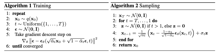
Training

1. Sample real data: Get a training image from your dataset
2. Random timestep: Choose how much noise to add (uniform across all levels)
3. Sample noise: Generate the specific noise to add
4. Create noisy version: Apply the forward process in one step
5. Predict noise: Ask the model “what noise was added?”
6. Update: Make the model better at noise prediction

• Single-step training: Instead of running the full T-step forward process, we can jump directly to any timestep t using the closed-form formula.
• Stochastic training: Each batch sees different noise levels, so the model learns to denoise across all levels simultaneously.
• Simple objective: Just predict noise - no complex distributions or adversarial training.

Connection to Score Matching

The noise prediction objective is equivalent to denoising score matching:

\[\nabla_{x_t} \log p(x_t) \approx -\frac{\varepsilon}{\sqrt{1 - \bar{\alpha}_t}}\]

What this means:

• Predicting noise \(\varepsilon\) is equivalent to predicting the gradient of the log-probability
• The model learns the “gradient field” pointing toward high-probability regions
• Sampling follows these gradients to find realistic images

Why this Matter?

• Theoretical foundation: Connects diffusion models to the rich theory of score-based generative models.
• Sampling interpretation: The reverse process becomes Langevin dynamics following learned gradients.
• Stability: Score matching is known to be more stable than adversarial training.

More

Variance Schedule Choice

The paper fixes the forward process variances \(β_t\) to constants rather than learning them.

• This simplification means the forward process q has no learnable parameters
• The term \(L_T\) becomes constant and can be ignored during training
  • Linear schedule: \(β_t\) increases linearly from \(β_1\) to \(β_T\)
  • Typical values: \(β_1 = 0.0001\), \(β_T = 0.02\)
  • T steps: Usually T = 1000 for training

Covariance Choice:

The model sets \(\Sigma_\theta(x_t,t) = \sigma_t^2 I\) (diagonal, time-dependent constants):

• \(\sigma_t^2 = \beta_t\): Optimal when \(x_0 \sim N(0,I)\)
• \(\sigma_t^2 = \tilde{\beta}_t\): Optimal when \(x_0\) is deterministic
• Both choices gave similar empirical results

Image Preprocessing:

• Images are scaled from {0,1,…,255} to [-1,1]
• Ensures consistent neural network input scaling
• Starting point is standard normal prior \(p(x_T)\)

Practical Implementation Details

• Training Tips:
  • EMA for sampling
  • Gradient clipping
  • Cosine learning rate schedule
  • Data augmentation

Experiments

Experiment Setup

• T = 1000: Number of diffusion steps, matching prior work to keep neural network evaluations comparable.
• Noise schedule: Linearly increasing variances from \(β_1 = 10^{-4}\) to \(β_T = 0.02\), which keeps added noise small but enough to reach near-complete destruction of the original signal by the end.
• Signal-to-noise control: Final KL divergence from Gaussian is \(\approx 10^{-5}\) bits/dim — ensures the model learns well.

Model Architecture

• U-Net: Based on unmasked PixelCNN++ with group normalization and shared weights across time.
• Time embeddings: Injected using Transformer sinusoidal embeddings.
• Self-attention: Added at 16×16 feature resolution.

Training Objective Ablation

• True Variational Bound: Best for compression (lossless codelength).
• Simplified Objective: Best for sample quality.
• Predicting mean \(\tilde{\mu}\):
  • Works well with variational bound.
  • Performs worse with simple MSE objective.
• Learned variance: Leads to instability and poor quality.
• Fixed variance: More stable.

Progressive Generation

• Generate images progressively from random bits (reverse process).
• Large-scale features appear early; details come later.
• Shows that Gaussian diffusion allows coarse-to-fine image generation.

Interpolation in Latent Space

• Interpolate two images in latent space (at same timestep t), then decode via reverse process.
• Results:
  • Smooth and meaningful transitions in pose, hair, background, etc.
  • Eyewear remains unchanged, showing model’s bias or lack of variation in that feature.
  • Larger t → blurrier but more varied (i.e., creative) results.

Connection to Autoregressive Models

• Rewriting the variational bound shows diffusion is like autoregressive decoding with a continuous and generalized bit ordering.
• Gaussian noise acts like masking but may be more natural and effective.
• Unlike true autoregressive models, diffusion can use T < data dimension, allowing flexibility in sampling speed or model power.

Key Takeaways

• Diffusion models:
  • Achieve high-quality image synthesis even without conditioning.
  • Show strong lossy compression ability (good perceptual reconstructions).
  • Can act as a generalization of autoregressive models.
• Model architecture and training objective greatly affect performance.
• Progressive generation, interpolation, and decoding are all efficient and visually plausible.