2025-05-28

DeepSeek-V3 Technical Report

These are the notes for the paper: DeepSeek-V3 Technical Report

Abstract

Model Architecutre

Transformer-based model

1. DeepSeekMoE

671B parameters with 37B activated for each token.
Architecture is same as v2

2. Multi-Head Latent Attention (MLA)

Look below

3. Auxiliary-loss-free strategy for load balancing (NEW)

Aim of minimizing the adverse impact on model performance that arises from the effort to encourage load balancing.

Data

Training

Setting

Low-precision training: FP8 mixed precision training framework
- Closely tied to the hardware
Design the DualPipe algorithm for efficient pipeline parallelism: model further scales up, as long as we maintain a constant computation-to-communication ratio
Efficient cross-node all-to-all communication kernels to fully utilize InfiniBand (IB) and NVLink bandwidths.

Multi-Token Prediction (MTP) training objective (NEW)

Enhance the overall performance on evaluation benchmarks.

Process:

Pretraining:
- Data: Pre-trained on 14.8T tokens
- Process:
  - Remarkably stable
  - Two-stage context length extension: 32K and 128K
Supervised Fine-Tuning and Reinforcement Learning stages
- Data:
- Process:
  - SFT: Supervised Fine-Tuning
  - RL: Reinforcement Learning
Post-training:
- Data:
- Process:
  - Distill the reasoning capability from the DeepSeekR1 series of models, and meanwhile carefully maintain the balance between model accuracy

Multi-Head Latent Attention

Background: Rotary Positional Embeddings (RoPE)

Before diving into Multi-Head Latent Attention, it’s crucial to understand Rotary Positional Embeddings (RoPE), as they play a key role in why MLA’s design is necessary and elegant.

What is RoPE?

RoPE (Rotary Positional Embedding) encodes positional information through rotation matrices applied to token embeddings. Unlike absolute positional encodings, RoPE allows models to learn relative positional relationships implicitly, making it highly effective for long-context understanding.

In Rotary Positional Embeddings (RoPE), the embedding dimension $D$ is divided into pairs of features, and each pair undergoes a 2D rotation transformation.

Understanding the Feature Pairing

What is $i$?

$i$ is the feature index in the embedding dimension $D$. Since RoPE operates on feature pairs, the indices are divided into even-odd index pairs: $(x_0, x_1), (x_2, x_3), (x_4, x_5), \ldots, (x_{D-2}, x_{D-1})$

The index $i$ iterates over half of the embedding dimensions, i.e., from $i = 0$ to $i = D/2 - 1$.

Why Pair Features?

Each token embedding $x \in \mathbb{R}^D$ is not rotated as a whole but instead divided into 2D subspaces, where each pair of values represents coordinates in a 2D plane. This allows the model to encode positional information using a rotation matrix:

\[\begin{bmatrix} x_{2i}^{(p)} \\ x_{2i+1}^{(p)} \end{bmatrix} = \begin{bmatrix} \cos(\theta_p) & -\sin(\theta_p) \\ \sin(\theta_p) & \cos(\theta_p) \end{bmatrix} \begin{bmatrix} x_{2i} \\ x_{2i+1} \end{bmatrix}\]

The Rotation Mechanism

For each feature pair $(x_{2i}, x_{2i+1})$:

$x_{2i}$ and $x_{2i+1}$ are treated as 2D coordinates
These coordinates are rotated by an angle $\theta_p$ specific to the position $p$
The rotation encodes positional information directly into the embedding values

Expanded Rotation Calculation:

Using trigonometric expansion:

\[\begin{aligned} x_{2i}^{(p)} &= x_{2i} \cos(\theta_p) - x_{2i+1} \sin(\theta_p) \\ x_{2i+1}^{(p)} &= x_{2i} \sin(\theta_p) + x_{2i+1} \cos(\theta_p) \end{aligned}\]

This ensures that:

Lower-dimensional embeddings rotate slower (longer wavelength)
Higher-dimensional embeddings rotate faster (shorter wavelength)
The model learns relative positional information instead of absolute positions

Rotation Angle Formula

The rotation angle per feature is:

\[\theta_p = \frac{p}{10000^{2i/D}}\]

Example Calculation for $D = 1024$:

Given:

$D = 1024$, so there are 512 feature pairs
$p$ is the token position
$i = 0, 1, \ldots, 511$

For position $p = 10$ and feature pair $i = 100$:

\[\theta_{10} = \frac{10}{10000^{200/1024}}\]

Applying to embedding pair $(x_{200}, x_{201})$:

\[\begin{aligned} x_{200}^{(10)} &= x_{200} \cos(\theta_{10}) - x_{201} \sin(\theta_{10}) \\ x_{201}^{(10)} &= x_{200} \sin(\theta_{10}) + x_{201} \cos(\theta_{10}) \end{aligned}\]

How RoPE Preserves Inner Products in Attention

One of the key mathematical advantages of RoPE is that it preserves the inner product between queries ($Q$) and keys ($K$) after applying rotations. This means the self-attention mechanism remains unchanged, while relative positional information is encoded.

Inner Products in Self-Attention

In a standard Transformer, the self-attention scores are computed as:

\[\text{Attention}(Q, K, V) = \text{softmax}\left(\frac{QK^T}{\sqrt{D}}\right)V\]

where:

$Q$ (Query) and $K$ (Key) are embeddings of shape (Batch, Sequence Length, Embedding Dimension)
$K^T$ is the transposed matrix of $K$
$D$ is the embedding dimension

The core operation in attention is the dot product $Q \cdot K^T$, which determines how similar two tokens are.

How RoPE Affects Queries and Keys

With RoPE, we replace the standard $Q$ and $K$ embeddings with their rotated versions:

\[Q_p' = R_\theta(p) \cdot Q_p, \quad K_q' = R_\theta(q) \cdot K_q\]

where:

$R_\theta(p)$ and $R_\theta(q)$ are rotation matrices applied to positions $p$ and $q$
These rotations encode the positional information without modifying the fundamental geometric properties of dot products

Preserving the Inner Product

The key mathematical property of rotation matrices is:

\[R_\theta(p) R_\theta(q)^{-1} = R_\theta(p-q)\]

This means that when computing the dot product between the rotated queries and keys:

\[\langle Q_p', K_q' \rangle = \langle R_\theta(p) Q_p, R_\theta(q) K_q \rangle\]

Using the rotation property:

\[\langle R_\theta(p) Q_p, R_\theta(q) K_q \rangle = \langle R_\theta(p-q) Q_p, K_q \rangle\]

Thus, the attention score now includes relative positional information:

\[Q_p' \cdot K_q'^T = (R_\theta(p) Q_p) \cdot (R_\theta(q) K_q)^T\]

Since rotation does not change vector norms or inner products, the self-attention mechanism remains functionally unchanged.

Why This Matters

Preserving Inner Product → The Transformer does not need modifications to compute attention
Relative Position Encoding → The difference $R_\theta(p-q)$ captures relative positions, unlike absolute embeddings
Stable Attention Computation → Unlike learned positional embeddings, RoPE does not interfere with how attention weights are computed

RoPE: Deriving the Inner Product Identity

The Key Step: How We Get $\langle R_\theta(p)Q_p, R_\theta(q)K_q\rangle = \langle R_\theta(p-q)Q_p, K_q\rangle$

Starting Point

We begin with the inner product of two rotated vectors: $\langle R_\theta(p)Q_p, R_\theta(q)K_q\rangle$

Step 1: Express as Matrix Multiplication

The inner product can be written as: $\begin{aligned} \langle R_\theta(p)Q_p, R_\theta(q)K_q\rangle &= (R_\theta(p)Q_p)^T (R_\theta(q)K_q) \\ &= Q_p^T R_\theta(p)^T R_\theta(q) K_q \end{aligned}$

Step 2: Use Orthogonal Property of Rotation Matrices

For rotation matrices, we have the crucial property: $R_\theta(p)^T = R_\theta(p)^{-1} = R_\theta(-p)$

This is because rotation matrices are orthogonal matrices.

Substituting: $Q_p^T R_\theta(p)^T R_\theta(q) K_q = Q_p^T R_\theta(-p) R_\theta(q) K_q$

Step 3: Apply Rotation Composition Property

Rotations compose by adding their angles: $R_\theta(-p) R_\theta(q) = R_\theta(-p + q) = R_\theta(q - p)$

So we get: $Q_p^T R_\theta(q - p) K_q$

Step 4: Connect to the Target Expression

Now, let’s look at what we want to show equals this: $\langle R_\theta(p-q)Q_p, K_q\rangle = (R_\theta(p-q)Q_p)^T K_q = Q_p^T R_\theta(p-q)^T K_q$

Using the orthogonal property again: $R_\theta(p-q)^T = R_\theta(-(p-q)) = R_\theta(q-p)$

Therefore: $\langle R_\theta(p-q)Q_p, K_q\rangle = Q_p^T R_\theta(q-p) K_q$

Final Result

We’ve shown that: $\langle R_\theta(p)Q_p, R_\theta(q)K_q\rangle = Q_p^T R_\theta(q-p) K_q = \langle R_\theta(p-q)Q_p, K_q\rangle$

Key Properties Used

Orthogonal Property: $R_\theta^T = R_\theta^{-1} = R_{-\theta}$
Composition Property: $R_{\theta_1} R_{\theta_2} = R_{\theta_1 + \theta_2}$
Inner Product Definition: $\langle x, y\rangle = x^T y$

Why This Matters for RoPE

This identity shows that the attention score between positions $p$ and $q$ depends only on their relative distance $(p-q)$, not their absolute positions. This is exactly what we want for relative position encoding!

The attention mechanism becomes: $\text{Attention}(p,q) \propto \langle R_\theta(p-q)Q_p, K_q\rangle$

This preserves the translational invariance property while encoding relative positional relationships.

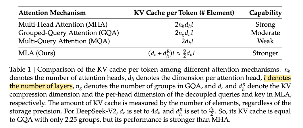
0. Recap of the attention family

Variant	What changes?	KV-cache size
MHA (Multi-Head Attention)	Each of the $h$ heads owns its own $W_q,W_k,W_v$.	Large – grows with $h$.
MQA (Multi-Query Attention)	All heads share one $K$ and one $V$.	Small – only one pair stored.
GQA (Grouped-Query Attention)	Heads are split into $g$ groups; heads inside a group share one $K,V$.	In-between MHA and MQA.

The goal of MLA (Multi-head Latent Attention) is: “match or beat GQA’s quality while making the KV-cache as small as possible.”

1. Low-rank projection is not the real novelty

The DeepSeek-V2 report introduces MLA through low-rank projection. But low rank already hid inside GQA! Stack every group’s key and value:

\[\underbrace{\bigl[k^{(1)}_i,\dots,k^{(g)}_i,\;v^{(1)}_i,\dots,v^{(g)}_i\bigr]}_{c_i\in\mathbb R^{g(d_k+d_v)}} =\;x_i\; \underbrace{\bigl[W^{(1)}_k,\dots,W^{(g)}_k,\;W^{(1)}_v,\dots,W^{(g)}_v\bigr]}_{W_c\in\mathbb R^{d\times g(d_k+d_v)}} .\]

Because $g(d_k+d_v)!<!d$, the map $x_i!\mapsto!c_i$ is already a low-rank projection. So MLA’s real contribution is what happens after that projection.

2. Part 1 – Adding flexibility without enlarging the cache

2.1 Naïve idea: give each head its own linear transforms again

After the shared low-rank step $x_i!\to!c_i$, let every head use its own $W_k^{(s)},W_v^{(s)}$ instead of GQA’s cut-and-copy trick:

\[\begin{aligned} q_t^{(s)} &= x_t\,W_q^{(s)} \quad &&\in\mathbb R^{d_k},\\ k_i^{(s)} &= c_i\,W_k^{(s)} \quad &&\in\mathbb R^{d_k},\\ v_i^{(s)} &= c_i\,W_v^{(s)} \quad &&\in\mathbb R^{d_v},\\ o_t^{(s)} &= \mathrm{Attention}\bigl(q_t^{(s)}, k_{\le t}^{(s)}, v_{\le t}^{(s)}\bigr). \end{aligned}\tag{5}\]

Problem: all heads have distinct $k_i^{(s)},v_i^{(s)}$ again ⇒ KV-cache balloons back to MHA size.

2.2 Trick: merge the two matrices at inference time

Observe the dot product inside soft-max:

\[q_t^{(s)}\;k_i^{(s)\!\top} \;=\;(x_t W_q^{(s)})\,(c_i W_k^{(s)})^\top \;=\;x_t\;\bigl(W_q^{(s)}\,W_k^{(s)\!\top}\bigr)\;c_i^{\!\top}. \tag{6}\]

At inference we can pre-multiply $W_q^{(s)}W_k^{(s)!\top}$ once and treat it as a single projection for $Q$. Then we store only $c_i$ (shared by all heads) in the KV-cache. Hence MLA decodes with the same cache size as GQA but owns more expressive per-head transforms during training.

2.3 Further cache shrink: choose an even smaller latent size $d_c$

Because only $c_i$ is cached, pick

\[d_c < g(d_k+d_v)\quad(\text{DeepSeek-V2 uses }d_c=512)\]

to compress the cache below GQA size.

Numerical caveat: The exact merge $W_q^{(s)}W_k^{(s)!\top}$ is precise only in infinite-precision math. With bf16 / fp16 kernels the extra multiply can lose accuracy, but empirical loss is acceptable.

3. Part 2 – The RoPE incompatibility and the fix

3.1 Why merge fails with RoPE

Rotary position embedding inserts a position-dependent matrix $R_m$ (block-diag, size $d_k\times d_k$) such that $R_m R_n^\top=R_{m-n}$.

With RoPE the dot product becomes

\[q_t^{(s)}k_i^{(s)\!\top} =(x_t W_q^{(s)} R_t)\,(c_i W_k^{(s)} R_i)^\top = x_t \bigl(W_q^{(s)} R_{t-i} W_k^{(s)\!\top}\bigr) c_i^{\!\top}. \tag{7}\]

Because $R_{t-i}$ depends on $(t-i)$, we cannot pre-merge $W_q^{(s)}$ and $W_k^{(s)}$ into one constant matrix—merging fails.

3.2 Tried work-arounds

Drop RoPE and switch to ALiBi – hurts quality.
Use Sandwich bias – still a compromise.
Stick $R_i$ after the low-rank projection ($q_i=c_i R_i$) – keeps absolute info only, loses relative formulation.

3.3 Final MLA compromise: dedicate a small RoPE sub-space

Let every head hold an extra $d_r$-dim block that carries RoPE, while the main $d_k$-dim part stays merge-friendly. Keys receive those RoPE dims once per group (shared across heads), so cache cost is tiny.

\[\begin{aligned} q_i^{(s)} &= \bigl[c_i W_{qc}^{(s)},\;\; c_i W_{qr}^{(s)} R_i\bigr] &&\in\mathbb R^{d_k+d_r},\\ k_i^{(s)} &= \bigl[c_i W_{kc}^{(s)},\;\; x_i W_{kr}^{(s)} R_i\bigr] &&\in\mathbb R^{d_k+d_r},\\ v_i^{(s)} &= c_i W_v^{(s)} &&\in\mathbb R^{d_v}. \tag{9} \end{aligned}\]

DeepSeek-V2 sets $d_r = d_k/2 = 64$. Only the K-cache grows by $d_r$.

4. Part 3 – Low-rank Q as well & the two-phase runtime

To save training RAM, MLA also turns $Q$ into a low-rank path with its own width $d’_c$ (DeepSeek-V2 uses $d’_c=1536$, different from $d_c=512$):

\[c'_i = x_i W'_c \in\mathbb R^{d'_c}, \qquad q_i^{(s)} = \bigl[c'_i W_{qc}^{(s)},\; c'_i W_{qr}^{(s)} R_i\bigr]. \tag{10}\]

4.1 Training (prefill) phase

Run the full “MHA-like” form (10). Parallelism across the whole prompt hides the extra inner products.

4.2 Decoding (generation) phase

Switch to MQA-like form by merging matrices exactly as in §2.2; only one $c_i$ is cached:

\[\begin{aligned} k_i &= \bigl[c_i,\;x_i W_{kr}^{(s)} R_i\bigr] \in\mathbb R^{d_c+d_r},\\ \text{V-head size} &= d_c \quad(\text{≈ 4× vanilla }d_v). \tag{12} \end{aligned}\]

Compute per token is heavier than plain MQA but the bottleneck now is memory-bandwidth, so generation speed still climbs markedly.

5. Consequences for model size & speed

KV-cache: scales with $d_c!+!d_r$, independent of head count $h$.
DeepSeek-V2 therefore cranks heads up to $h=128$ while keeping $d_k=128$ and model hidden size $d=5120$. More heads ⇒ more capacity with zero cache penalty.

6. Summary

MLA’s essence Low-rank latent $c_i$+ per-head linear maps ⇒ richer than GQA, but at inference we merge matrices so only $c_i$ is cached.
RoPE issue & fix Full merge breaks with RoPE; MLA reserves a small RoPE sub-space ($d_r$), shared in $K$, which adds minimal cache overhead.
Two-phase execution Training / prefill: wide, MHA-style. Generation: merged, MQA-style ⇒ lower bandwidth need and faster decoding.
Practical knobs (DeepSeek-V2) $d_c=512,\;d_r=64,\;d’_c=1536,\;d_k=128,\;h=128$.

MLA therefore delivers MHA-level quality, GQA-level (or better) cache, and faster generation, which is why it underpins the speed/quality trade-offs in DeepSeek-V2.

7. A Clearer Walkthrough: MLA in Simple Terms

7.1. Classic multi-head attention (MHA) in one minute

For every token vector $x_i\in\mathbb R^{d}$

\[\begin{aligned} Q_i^{(s)} &= x_i W_q^{(s)} \in \mathbb R^{d_k},\\ K_i^{(s)} &= x_i W_k^{(s)} \in \mathbb R^{d_k},\\ V_i^{(s)} &= x_i W_v^{(s)} \in \mathbb R^{d_v}, \end{aligned} \qquad s=1\dots h.\]

Each head $s$ has its own three matrices, so every token writes $h$ distinct $K$ and $h$ distinct $V$ blocks into the KV-cache.

Memory per token $\displaystyle \text{MHA_cache} = h\,(d_k+d_v)$.

7.2. Latent step that MLA (and already GQA) starts with

Project the long state $x_i$ down to a latent vector:
\[c_i = x_i W_c,\qquad W_c\in\mathbb R^{d\times d_c},\; d_c\ll d.\]
During training each head learns its own small maps:
\[K_i^{(s)} = c_i W_k^{(s)},\quad V_i^{(s)} = c_i W_v^{(s)}.\]

Because $d_c<d$, $W_c$ is already a low-rank projection; that part is not new.

7.3. Where the merging trick appears

7.3a. Look inside the attention dot product

\[\underbrace{Q_t^{(s)}}_{x_t W_q^{(s)}} \;\cdot\; \underbrace{K_i^{(s)}}_{c_i W_k^{(s)}}^{\!\!\top} \;=\; x_t\; \bigl(W_q^{(s)}\,W_k^{(s)\!\top}\bigr) \;c_i^{\!\top}.\]

The two head-specific matrices multiply each other and become one composite matrix

\[M^{(s)}\;=\;W_q^{(s)} W_k^{(s)\!\top}\in\mathbb R^{d\times d_c}.\]

7.3b. What MLA does with that fact

Training (or “prefill”) phase – keep everything separate; this gives each head its extra freedom.
Generation phase – pre-compute $M^{(s)}$ once and:
- build queries as $Q_t^{(s)} = x_t M^{(s)}$;
- reuse the shared latent $c_i$ itself as the key for every head.

Only the latents are cached:

\[\text{MLA\_cache}=d_c\quad(\text{independent of }h).\]

The per-head $W_v^{(s)}$ can likewise be folded into the final output projection, so values can also reuse $c_i$.

7.4. Side-by-side comparison

aspect	MHA	MLA after merging
Keys/values stored per token	$h$ distinct blocks	1 shared latent $c_i$
Cache size	$h(d_k+d_v)$	$d_c$ (often < GQA)
Extra maths at decode	None	One extra matrix–vector multiply for each head: $x_t M^{(s)}$
Where the saved memory comes from	—	All heads agree to read the same cached $c_i$

7.5. Why is this legal?

A dot product $xA\cdot yB = x(AB^\top)y^\top$ lets you push the two linear layers to one side as long as nothing position-dependent sits between them. That is why vanilla MLA can merge, but RoPE needs the small “side-car” block (the position rotation matrix breaks the simple factorisation).

7.6. Practical upshot

Training feels like a beefed-up GQA: more expressive heads, still moderate memory.
Decoding feels like an MQA variant: tiny KV-cache, bandwidth-friendly, yet keeps most of the extra modelling power it learned.

The “whole merging” is therefore just the algebraic observation that two per-head matrices can be multiplied once and for all, letting every head read the same compact latent key/value that was already present in GQA, while classic MHA has no way to do this and must cache every head’s keys and values separately.

Standard Multi-Head Attention

$d$ be the embedding dimension,
$n_h$ the number of attention heads,
$d_h = d / n_h$ the dimension of each head, and
$\mathbf h_t \in \mathbb R^{d}$ the hidden-state input for the $t$-th token at this attention layer.

Linear projections

\[\begin{aligned} \mathbf q_t &= W_Q \mathbf h_t,\\ \mathbf k_t &= W_K \mathbf h_t,\\ \mathbf v_t &= W_V \mathbf h_t, \end{aligned}\]

where $W_Q, W_K, W_V \in \mathbb R^{d_h n_h \times d}$.

Head-wise splitting

\[\begin{aligned} \mathbf q_t &= [\mathbf q_{t,1}; \mathbf q_{t,2}; \dots; \mathbf q_{t,n_h}],\\ \mathbf k_t &= [\mathbf k_{t,1}; \mathbf k_{t,2}; \dots; \mathbf k_{t,n_h}],\\ \mathbf v_t &= [\mathbf v_{t,1}; \mathbf v_{t,2}; \dots; \mathbf v_{t,n_h}], \end{aligned}\]

with $\mathbf q_{t,i}, \mathbf k_{t,i}, \mathbf v_{t,i} \in \mathbb R^{d_h}$ for each head $i$.

Scaled-dot-product attention (per head)

\[\mathbf o_{t,i} = \sum_{j=1}^{t} \operatorname{Softmax}_j\!\left( \frac{\mathbf q_{t,i}^{\top} \mathbf k_{j,i}}{\sqrt{d_h}} \right)\mathbf v_{j,i}.\]

Concatenation & output projection

\[\mathbf u_t = W_O\,[\mathbf o_{t,1}; \mathbf o_{t,2}; \dots; \mathbf o_{t,n_h}],\]

where $W_O \in \mathbb R^{d \times d_h n_h}$.

During inference, all key–value (KV) tensors must be cached. For a sequence of length $\ell$, this consumes $2 n_h d_h \ell$ floating-point elements—often the chief memory bottleneck that constrains both batch size and maximum context length.

8. Why RoPE breaks the “merge-the-matrices” trick—and how MLA fixes it

(A step-by-step story that ties every moving part together.)

8.1. Recap: how the merge works without position encoding

For one head $s$

\[Q_t^{(s)}=x_t W_q^{(s)},\qquad K_i^{(s)}=c_i W_k^{(s)}.\]

Inside the attention score:

\[Q_t^{(s)} K_i^{(s)\!\top} = (x_t W_q^{(s)})(c_i W_k^{(s)})^{\!\top} = x_t\; \bigl( W_q^{(s)} W_k^{(s)\!\top}\bigr)\; c_i^{\!\top}.\]

Because the two matrices have no token-dependent term between them, we can pre-multiply them once

\[M^{(s)} := W_q^{(s)} W_k^{(s)\!\top},\]

replace every query by $x_t M^{(s)}$, and reuse the same latent $c_i$ for all heads. That is the whole merge.

8.2. What Rotary Position Embedding (RoPE) adds

RoPE multiplies every key and query with a position-specific rotation matrix $R_m$ (block-diagonal, orthogonal, and crucially: $R_m R_n^{!\top}=R_{m-n}$).

\[Q_t^{(s)} = x_t W_q^{(s)} R_t,\qquad K_i^{(s)} = c_i W_k^{(s)} R_i.\]

Now the score reads

\[(x_t W_q^{(s)} R_t)\,(c_i W_k^{(s)} R_i)^{\!\top} = x_t\;\bigl(W_q^{(s)} R_{t-i} W_k^{(s)\!\top}\bigr)\;c_i^{\!\top}.\]

Problem: the middle term contains $R_{t-i}$, which changes for every pair of positions. Therefore we cannot collapse $W_q^{(s)}$ and $W_k^{(s)}$ into one constant matrix—merging fails.

8.3. Straightforward but disappointing work-arounds

Idea	What happens	Drawback
Drop RoPE, use ALiBi or no bias	Merge works again	Empirically lower accuracy
Move RoPE to the latent: $c_iR_i$	Merge works	Only absolute positions injected → model must learn relativity from scratch

8.4. MLA’s elegant compromise: a tiny “RoPE side-car”

Split every head’s channel space
- Main block: $d_k$ dims → keeps merge trick, no RoPE.
- Side-car block: $d_r!\ll!d_k$ dims → carries RoPE.
Form the vectors

\[\begin{aligned} Q_i^{(s)} &= \bigl[c_i W_{qc}^{(s)},\;\; c_i W_{qr}^{(s)} R_i\bigr],\\ K_i^{(s)} &= \bigl[c_i W_{kc}^{(s)},\;\; x_i W_{kr}^{(s)} R_i\bigr],\\ V_i^{(s)} &= c_i W_v^{(s)}. \end{aligned}\]

The first half (no RoPE) still lets us merge $W_{qc}^{(s)}W_{kc}^{(s)!\top}$.
The side-car keeps relative position information.

Cache impact is tiny

All heads share the same side-car key block (it is computed from $x_i$, not $c_i$), so KV-cache grows by just $d_r$, not by $h!\times!d_r$.
In DeepSeek-V2: $d_k=128,\;d_r=64$. The cache per token is $d_c+d_r=512+64$ ≪ classic MHA’s $h(d_k+d_v)$.

8.5. Why accuracy survives

The model still receives high-resolution relative positions in the side-car.
The bigger main block (merge-able) focuses on content; the small block supplies position cues.
Experiments (DeepSeek-V2) show a negligible drop VS full-RoPE MHA with a 3–4 × memory win during decoding.

8.6. Putting it next to classic MHA

Feature	MHA + RoPE	MLA + side-car RoPE
Per-head matrices	$W_q^{(s)},W_k^{(s)},W_v^{(s)}$	Same during training
Can merge $W_qW_k^{!\top}$?	❌ (RoPE blocks it)	✅ for the $d_k$ main block
Cache per token	$h(d_k+d_v)$	$d_c+d_r$ (independent of $h$)
Position capacity	Full $d_k$ dims	Slim $d_r$ dims (64 of 192)
Empirical quality	Baseline	Matches baseline within noise

Take-away

RoPE injects a position-dependent rotation that makes the simple “multiply the two matrices once” trick impossible. MLA sidesteps the obstacle by cordoning off a small, shared sub-space to carry the rotation, letting the vast majority of each head merge cleanly—so the KV-cache stays small and the model still understands token order.

Comparison of the KV cache

MTP

DeepSeek-V3 Multi-Token Prediction: Complete Explanation

Core Concept

Standard Language Modeling

In standard language modeling, the model predicts only the next immediate token at each step:

Input: “The cat sat on the”
Predictions:
- Position 1 (“The”) → predict “cat”
- Position 2 (“cat”) → predict “sat”
- Position 3 (“sat”) → predict “on”
- Position 4 (“on”) → predict “the”

Multi-Token Prediction (MTP)

In Multi-Token Prediction, the model predicts multiple future tokens from each position:

Input: “The cat sat on the mat”
Predictions:
- Position 1 (“The”) → predict next tokens: “cat”, “sat”, “on”
- Position 2 (“cat”) → predict next tokens: “sat”, “on”, “the”
- Position 3 (“sat”) → predict next tokens: “on”, “the”, “mat”

Key Insight: MTP provides multiple training signals per position, thus increasing learning efficiency and promoting better internal planning.

Benefits of MTP

Denser Training Signals

Standard approach: 1 prediction per token.
MTP (e.g., 3-step prediction): 3 predictions per token, offering richer learning opportunities.

Improved Representation and Planning

MTP encourages the model to learn representations effective for predicting multiple future tokens, fostering better long-term dependency understanding and internal planning.

DeepSeek’s Sequential MTP Architecture

Architecture Overview

DeepSeek employs sequential modules rather than parallel heads:

Main Model → MTP Module 1 → MTP Module 2 → MTP Module 3
    ↓            ↓              ↓              ↓
Predict t+1   Predict t+2   Predict t+3   Predict t+4

Each MTP module includes:

Shared Embedding (from main model)
Shared Output Head (from main model)
Unique Transformer Block (specific to the prediction depth)
Projection Matrix (combines previous representations with actual tokens)

Step-by-Step Example

Input: “The cat sat on the mat”

Step 1: Main Model

Processes sequence, produces hidden representations (h^0_1, h^0_2, h^0_3, h^0_4, h^0_5).
Predicts next immediate tokens.

Step 2: MTP Module 1 (Predict t+2)

Position 1 (“The”): combines representation (h^0_1) and embedding of actual next token (“cat”), predicts “sat”.
Position 2 (“cat”): combines (h^0_2) and “sat” embedding, predicts “on”.

Step 3: MTP Module 2 (Predict t+3)

Builds upon Module 1’s representation. Position 1 takes Module 1’s representation and actual token embedding two steps ahead (“sat”) to predict “on”.

This sequential process maintains causality using actual ground-truth tokens, avoiding error propagation.

Maintaining Causality

Each MTP module uses actual tokens (not predictions), ensuring stable and accurate training:

Incorrect method (error-prone): using previous module predictions (“dog” instead of actual “cat”).
Correct method: always using actual tokens, ensuring modules learn from true signals.

Training Objective

Compute cross-entropy loss for each MTP module:

\[L_k^{\text{MTP}} = \text{CrossEntropy}(\text{predictions}_{k}, \text{targets}_{k})\]

where $k$ represents the prediction depth (1, 2, 3, …, $D$).

The aggregate MTP loss is:

\[L_{\text{MTP}} = \lambda \cdot \frac{1}{D} \sum_{k=1}^{D} L_k^{\text{MTP}}\]

where:

$\lambda$ is a weighting factor
$D$ is the maximum prediction depth
$L_k^{\text{MTP}}$ is the loss for predicting $k$ steps ahead

Module Size and Structure

Main Model: Large transformer (e.g., 600B parameters)
MTP Modules: Lightweight, single-transformer blocks (~1-2B parameters each), sharing embedding and output head with the main model.

Sequential vs. Parallel

Parallel (less effective): multiple independent heads, no contextual build-up.
Sequential (DeepSeek): each module builds on the previous representation, preserving causal structure and providing richer context.

Training vs. Inference

Training: Utilize all MTP modules for enhanced learning signals.
Inference: Optionally discard or repurpose modules for speculative decoding (accelerated inference).

Key Advantages

Enhanced Data Efficiency: More training signals per sequence.
Superior Planning: Better long-term dependency understanding.
Flexible Inference: Modules can be optionally used to accelerate inference.

Analogy

Main Model: A full orchestra.
MTP Modules: Small jazz ensembles borrowing instruments from the orchestra, adding short solos.

This elegant design ensures efficient, accurate, and flexible language modeling, enhancing both training effectiveness and inference speed.

Speculative Decoding: Complete Technical Guide

The Fundamental Problem

Standard Autoregressive Generation generates tokens sequentially, causing significant latency:

Input: "Write a Python function to"
Step 1: Generate "calculate" → 50ms
Step 2: Generate "the" → 50ms
Step 3: Generate "factorial" → 50ms
Step 4: Generate "of" → 50ms
Step 5: Generate "a" → 50ms
Total: 250ms for 5 tokens

Issue: Sequential token generation prevents parallelization, slowing down real-time applications significantly.

GPU Utilization: Typically very low (~10-20%), as GPUs remain idle during token waits, causing inefficient resource usage.

Core Idea of Speculative Decoding

Idea: Speculatively predict multiple tokens simultaneously using a faster but less accurate model, then verify all predictions concurrently using a more accurate but slower model:

Step 1: Small model speculates: "calculate the factorial of a number"
Step 2: Large model verifies simultaneously: ✓✓✓✓✗✗
Step 3: Accept first 4 tokens, reject the last 2, then continue.

Insight: Verification is highly parallelizable, leading to significant speed-ups.

Draft-Then-Verify Algorithm

Basic Procedure

Draft Generation: A small, fast model proposes multiple tokens.
Parallel Verification: A large, accurate model assesses each token simultaneously.
Acceptance/Rejection: Tokens are accepted based on probability ratios or replaced via rejection sampling.

Example Implementation

def speculative_decode(large_model, small_model, prompt, K, max_tokens=50):
    sequence = prompt
    while len(sequence) < max_tokens:
        draft_tokens = small_model.generate(sequence, num_tokens=K)
        extended_sequence = sequence + draft_tokens

        large_probs = large_model.get_probabilities(extended_sequence)
        small_probs = small_model.get_probabilities(extended_sequence)

        accepted_tokens = []
        for i, token in enumerate(draft_tokens):
            pos = len(sequence) + i
            accept_prob = min(1.0, large_probs[pos][token] / small_probs[pos][token])

            if random.random() < accept_prob:
                accepted_tokens.append(token)
            else:
                adjusted_probs = adjust_probabilities(large_probs[pos], small_probs[pos])
                next_token = sample_from_adjusted(adjusted_probs)
                accepted_tokens.append(next_token)
                break

        sequence += accepted_tokens

    return sequence

Step-by-Step Example

Prompt: “The capital of France is”
Small model drafts tokens, large model verifies:
- Draft: “Paris , which is”
- Large model verifies and accepts/rejects based on token probabilities.

Advanced Speculative Decoding Methods

Tree-Based Speculative Decoding

How it works: Construct multiple speculative paths (branches) simultaneously, forming a tree of possible sequences. The verification model then evaluates each path concurrently. The optimal path (highest likelihood or lowest perplexity) is selected and extended.

Parallel Sampling

How it works: Generate multiple distinct candidate sequences simultaneously using one or more small models. Each candidate is independently scored by the large verification model. The candidate with the highest verification score is chosen as the final output sequence.

Self-Speculative Decoding

How it works: Use a single model but with different generation settings. The model generates speculative tokens at low temperature (deterministic, focused predictions), and subsequently verifies them at higher temperature (more diverse and exploratory predictions). This approach leverages the strengths of a single model across varied settings.

Connection to Multi-Token Prediction (MTP)

MTP modules can naturally serve as speculative draft generators due to their trained capability to predict multiple tokens ahead.

Performance Analysis

Typical Speedups

Small drafts ($K = 2-4$): 2-3x
Medium drafts ($K = 8-16$): 3-5x
Large drafts ($K \geq 32$): Diminishing returns

Influencing Factors

Draft model quality
Sequence length
Task complexity
Model compatibility

Advanced Techniques

Lookahead Decoding

How it works: Multiple speculative continuations are generated with different random seeds. The verification model identifies and selects high-confidence prefixes common to these generated sequences, improving reliability and efficiency.

Confidence-Based Speculation

How it works: The speculation depth dynamically adjusts according to the confidence scores of the predictions. Speculation stops or reduces depth when confidence drops below a predefined threshold, ensuring balance between speed and accuracy.

Hierarchical Speculation

How it works: Speculative generation occurs through a hierarchy of progressively larger or more capable models. Initial rapid, coarse-grained predictions by smaller models are iteratively refined by more accurate, larger models. This ensures effective resource utilization and enhanced prediction accuracy.

Implementation Challenges

Memory Management

Efficient chunking and streaming methods mitigate increased memory use.

Load Balancing

Allocate computational resources asymmetrically (small model fewer GPUs, large model more GPUs).

Quality Control

Adjust speculation depth dynamically based on required quality.

Real-World Applications

Interactive Chat: Rapidly draft responses and verify in parallel for real-time interactions.
Code Generation: Generate structure with a small model, verify and complete details with a large model.

Limitations and Trade-offs

Quality Degradation: Potential decrease in output quality, requiring quality gating mechanisms.
Memory Overhead: Adaptive speculation depth based on available memory.
Model Compatibility: Draft and verification models need alignment to ensure consistency.

Future Directions

Learned Draft Models: Specialized models trained explicitly for drafting tasks.
Dynamic Speculation: Context-sensitive adjustment of speculation aggressiveness.
Multi-Modal Speculation: Incorporate other modalities (vision, audio) to improve text drafts.

Key Takeaways

Parallelize verification instead of sequential token generation.
Speed gains may trade off against quality.
Align models carefully for effective speculative decoding.
Adapt speculation strategies based on specific task contexts.
Speculative decoding significantly enhances real-time applicability of large models.

3. Infrastructures

3.1 Compute Clusters

DeepSeek-V3 is trained on a cluster equipped with 2048 NVIDIA H800 GPUs. Each node in the H800 cluster contains 8 GPUs connected by NVLink and NVSwitch within nodes. Across different nodes, InfiniBand (IB) interconnects are utilized to facilitate communications.

3.2 GPU Interconnects: NVLink, NVSwitch, and InfiniBand Explained

The Communication Problem in Large-Scale Training

When training massive models like DeepSeek-V3, you need thousands of GPUs working together. But GPUs need to constantly share information:

Problem: DeepSeek-V3 has 685B parameters
- Too big to fit on one GPU (H800 has 80GB memory)
- Need ~2048 GPUs working together
- GPUs must constantly exchange gradients, activations, parameters
- Communication becomes the bottleneck!

The Challenge: Moving data between GPUs fast enough that they’re not just waiting around.

DeepSeek-V3’s Hardware Setup

Total: 2048 NVIDIA H800 GPUs
Organization: 256 nodes × 8 GPUs per node

Each Node:
┌─────────────────────────────────────┐
│  GPU1  GPU2  GPU3  GPU4  GPU5  GPU6  GPU7  GPU8  │
│    \    |    |    /      \    |    |    /    │
│     \   |    |   /        \   |    |   /     │
│      \  |    |  /          \  |    |  /      │
│       \ |    | /            \ |    | /       │
│        NVSwitch Fabric (within node)        │
└─────────────────────────────────────┐
                    │
            InfiniBand Network
                    │
┌─────────────────────────────────────┐
│        Another Node...              │
│  8 more GPUs connected similarly    │
└─────────────────────────────────────┘

1. NVLink: GPU-to-GPU Highway

What is NVLink?

NVLink is NVIDIA’s proprietary high-speed interconnect that directly connects GPUs to each other.

Think of it as: A superhighway between GPUs, much faster than regular roads (PCIe).

Speed Comparison

PCIe 4.0: ~32 GB/s bidirectional
NVLink 4.0: ~900 GB/s bidirectional (28x faster!)

How NVLink Works

Traditional Setup (PCIe only):
GPU1 ↔ CPU ↔ GPU2
- All communication goes through CPU
- CPU becomes bottleneck
- Slow and inefficient

NVLink Setup:
GPU1 ↔ GPU2 (direct connection)
- GPUs talk directly to each other
- No CPU bottleneck
- Much faster data transfer

What NVLink Does in DeepSeek-V3 Training

1. Gradient Synchronization

# During backpropagation, GPUs need to share gradients
GPU1_gradients = compute_gradients(batch_1)
GPU2_gradients = compute_gradients(batch_2)

# Via NVLink: Super fast sharing
GPU1.send_gradients_to(GPU2)  # 900 GB/s transfer rate
GPU2.send_gradients_to(GPU1)

# Average the gradients for synchronized training
final_gradients = (GPU1_gradients + GPU2_gradients) / 2

2. Model Parallelism

# Different parts of the model on different GPUs
GPU1: Layers 1-10 of transformer
GPU2: Layers 11-20 of transformer
GPU3: Layers 21-30 of transformer

# Forward pass: Data flows through NVLink
input → GPU1 → [NVLink] → GPU2 → [NVLink] → GPU3 → output

3. Parameter Sharing

# Some parameters need to be accessed by multiple GPUs
shared_embeddings = load_on_GPU1()
GPU2.request_embeddings()  # Via NVLink
GPU3.request_embeddings()  # Via NVLink
# Much faster than going through CPU/system memory

2. NVSwitch: The Smart Traffic Controller

What is NVSwitch?

NVSwitch is a switching fabric that creates a full mesh network between multiple GPUs using NVLink.

Think of it as: A smart highway interchange that lets any GPU talk to any other GPU directly.

The Problem NVSwitch Solves

Without NVSwitch (simple NVLink connections):

8 GPUs, each with 4 NVLink connections:
GPU1 ↔ GPU2 ↔ GPU3 ↔ GPU4
 ↓       ↓       ↓       ↓
GPU5 ↔ GPU6 ↔ GPU7 ↔ GPU8

Problem: GPU1 talking to GPU8 needs multiple hops
GPU1 → GPU2 → GPU3 → GPU4 → GPU8 (slow, creates bottlenecks)

With NVSwitch:

     NVSwitch Fabric
    ┌─────────────────┐
GPU1 ┤                 ├ GPU5
GPU2 ┤                 ├ GPU6  
GPU3 ┤   All-to-All    ├ GPU7
GPU4 ┤   Connection    ├ GPU8
    └─────────────────┘

Result: Any GPU can talk to any other GPU in one hop!
GPU1 → NVSwitch → GPU8 (direct, fast)

NVSwitch in Action

1. Dynamic Load Balancing

# Model decides GPU4 is underutilized, GPU1 is overloaded
workload_rebalance()

# Via NVSwitch: Instant communication to any GPU
GPU1.send_work_to(GPU4)  # Direct path through NVSwitch
# No need to route through intermediate GPUs

2. Flexible Model Partitioning

# Can dynamically assign any layers to any GPUs
layer_assignment = {
    'attention_layers': [GPU1, GPU3, GPU7],  # Non-adjacent GPUs
    'ffn_layers': [GPU2, GPU4, GPU6],
    'embeddings': [GPU5, GPU8]
}

# NVSwitch enables efficient communication between any combination

3. All-Reduce Operations

def all_reduce_with_nvswitch(gradients):
    """
    All GPUs need to share and average their gradients
    """
    # Without NVSwitch: Ring topology, many steps
    # With NVSwitch: All GPUs can communicate simultaneously
    
    for gpu_pair in all_possible_pairs:
        # All exchanges happen in parallel via NVSwitch
        gpu_pair[0].exchange_gradients(gpu_pair[1])
    
    # Much faster than sequential ring-based all-reduce

3. InfiniBand: The Inter-Node Network

What is InfiniBand?

InfiniBand (IB) is a high-performance networking standard that connects different compute nodes together.

Think of it as: The highway system connecting different cities (nodes), where each city has 8 GPUs.

Why InfiniBand for DeepSeek-V3?

The Scale Challenge:

2048 GPUs total
256 nodes × 8 GPUs per node

Within each node: NVLink + NVSwitch (super fast)
Between nodes: Need network connection (InfiniBand)

InfiniBand Performance

Ethernet (typical): ~25 Gbps
InfiniBand HDR: ~200 Gbps (8x faster)
InfiniBand NDR: ~400 Gbps (16x faster)

Also: Much lower latency than Ethernet
- Ethernet: ~10-50 microseconds
- InfiniBand: ~1-5 microseconds

How InfiniBand Works

Traditional Ethernet:

Node1 → Router → Switch → Router → Node2
- Multiple hops
- Higher latency
- Packet processing overhead

InfiniBand:

Node1 → InfiniBand Switch → Node2
- Direct path
- Hardware-accelerated
- RDMA (Remote Direct Memory Access)

RDMA: The Secret Sauce

RDMA lets GPUs on different nodes access each other’s memory directly:

# Without RDMA (traditional networking)
def send_data_slow(data, target_node):
    # 1. Copy data from GPU to CPU memory
    cpu_buffer = gpu_to_cpu(data)
    # 2. Send via network stack (involves OS, drivers, etc.)
    network_send(cpu_buffer, target_node)
    # 3. Receive on target node, copy to GPU
    target_gpu = cpu_to_gpu(received_data)

# With RDMA via InfiniBand
def send_data_fast(data, target_node):
    # Direct GPU-to-GPU transfer across nodes!
    gpu_direct_transfer(data, target_node.gpu)
    # No CPU involvement, no OS overhead

InfiniBand in DeepSeek-V3 Training

1. Inter-Node Gradient Synchronization

# All 256 nodes need to synchronize gradients
for node in all_nodes:
    # Each node computes gradients from its 8 GPUs
    node_gradients = combine_gradients_from_8_gpus()
    
    # Share with all other nodes via InfiniBand
    broadcast_to_all_nodes(node_gradients)  # RDMA transfers

# Result: All 2048 GPUs have consistent gradients

2. Model Checkpointing

# Save model state across all nodes
def save_checkpoint():
    for node_id in range(256):
        node_parameters = collect_from_8_gpus(node_id)
        # Fast transfer to storage node via InfiniBand
        rdma_transfer(node_parameters, storage_node)

3. Pipeline Parallelism Across Nodes

# Different transformer layers on different nodes
Node1: Layers 1-10    (8 GPUs handling these layers)
Node2: Layers 11-20   (8 GPUs handling these layers)  
Node3: Layers 21-30   (8 GPUs handling these layers)
...

# Forward pass: activations flow between nodes
activation_data = Node1.compute_layers_1_to_10(input)
# InfiniBand transfer to next node
Node2.receive_activations(activation_data)
activation_data = Node2.compute_layers_11_to_20(activation_data)
# Continue pipeline...

The Complete Picture: How They Work Together

Data Flow in DeepSeek-V3 Training

Step 1: Within Each Node (NVLink + NVSwitch)

Input batch arrives at Node 1:
- Split across 8 GPUs via NVSwitch
- GPUs process in parallel using NVLink for communication
- Fast gradient sharing within the node

Step 2: Between Nodes (InfiniBand)

Node 1 completes its computation:
- Aggregated results sent to other nodes via InfiniBand
- All 256 nodes synchronize their gradients
- Parameter updates coordinated across all nodes

Step 3: The Training Loop

def deepseek_v3_training_step(batch):
    # Within each node: NVLink + NVSwitch
    for node in all_256_nodes:
        node_gradients = []
        for gpu in node.8_gpus:
            gpu_gradient = gpu.compute_gradient(batch_slice)
            # Share via NVLink to other GPUs in same node
            gpu.broadcast_gradient_via_nvlink(gpu_gradient)
            node_gradients.append(gpu_gradient)
        
        # Aggregate gradients within node using NVSwitch
        node.aggregate_gradients_via_nvswitch(node_gradients)
    
    # Between nodes: InfiniBand
    global_gradients = []
    for node in all_256_nodes:
        # Send node's aggregated gradients to all other nodes
        node.broadcast_via_infiniband(node.aggregated_gradients)
        global_gradients.append(node.aggregated_gradients)
    
    # Final synchronization
    final_gradient = average(global_gradients)
    
    # Update model parameters (synchronized across all 2048 GPUs)
    update_parameters(final_gradient)

Why This Architecture Matters

Performance Benefits

Without Advanced Interconnects:

Training time: ~6 months (hypothetical)
Bottleneck: 90% waiting for communication
GPU utilization: ~10%

With NVLink + NVSwitch + InfiniBand:

Training time: ~2 months (actual)
Communication overhead: ~10%
GPU utilization: ~80-90%

Scaling Efficiency

Traditional PCIe + Ethernet scaling:
- 2x GPUs → 1.3x performance (poor scaling)
- Communication bottlenecks dominate

NVLink + NVSwitch + InfiniBand scaling:
- 2x GPUs → 1.8x performance (good scaling)
- Communication keeps up with computation

Cost and Complexity

Hardware Investment

Cost per H800 GPU: ~$25,000
NVLink/NVSwitch: Included in GPU cost
InfiniBand Infrastructure: ~$2,000 per node

Total for DeepSeek-V3:
- GPUs: 2048 × $25,000 = $51.2M
- InfiniBand: 256 × $2,000 = $0.5M
- Total: ~$52M in hardware

Why It’s Worth It

Training DeepSeek-V3 without proper interconnects:

Would take 3-4x longer
Higher energy costs
Opportunity cost of delayed model release
Total cost: Actually higher despite cheaper hardware

With proper interconnects:

Faster training
Better GPU utilization
Quicker time to market
Better ROI despite higher upfront cost

Key Takeaways

NVLink: Superhighway between GPUs within a node (~28x faster than PCIe)
NVSwitch: Smart traffic controller enabling any-to-any GPU communication
InfiniBand: High-speed network connecting nodes with RDMA capabilities
Together: They create a unified computing fabric that makes 2048 GPUs work like one giant computer
Result: DeepSeek-V3 training becomes feasible in reasonable time

The interconnect technology is just as important as the GPUs themselves - without it, you’d have 2048 very expensive paperweights waiting around for data to transfer!